Chapter 10: Multifactorial analyses using R
Figure 10.1 Output for one- way analysis of variance
Box 10.3 Presenting the results for one-way analysis of variance
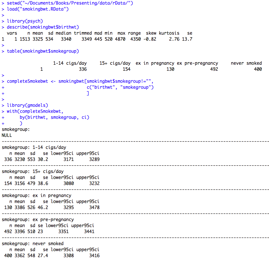
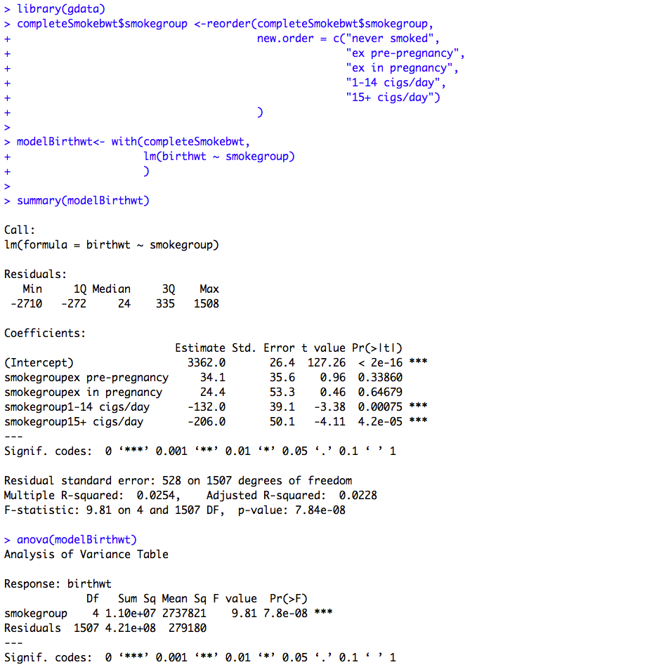
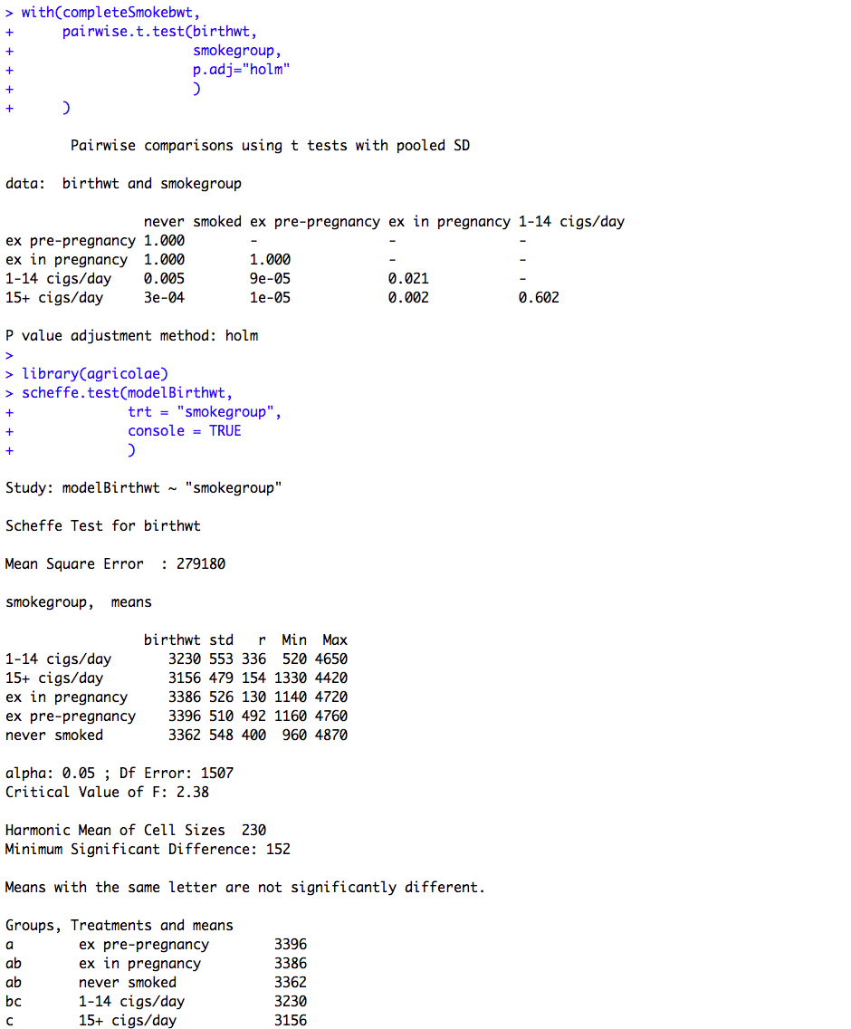
Figure 10.1 and Box 10.3 Code
Click here to show code with comments# Tell R where you will be working. R will look here for your data: setwd("~/Documents/Books/Presenting/data/rData/") # See chapter 2 for more details on the setwd() function. # Use the load() function to load the dataset smokingbwt.RData out of the # current folder/directory into R's interactive working memory/environment. See # chapter 2 for more details. load("smokingbwt.RData") # Use the library() package to load the psych package for the describe() # function. See chapter 2 for more details on library(). library(psych) # The describe() function in the psych package does descriptive statistics # including a standard deviation. See chapter 2 for more details. describe(smokingbwt$birthwt) # Look for bad/impossible data. # The table() function does simple cross tabulation tables. table(smokingbwt$smokegroup) # Check for empty factor levels. # Make a dataset that has the two variables and drops the record # with the factor level of "". "" is a legal value so the complete.cases() function # will not drop the blank. The syntax is: # dataframe[ what records , what columns ] completeSmokebwt <- smokingbwt[smokingbwt$smokegroup!="", c("birthwt", "smokegroup") ] library(gmodels) # Load the gmodels package for the ci() function. # See chapter 2 for details on the with() function. with(completeSmokebwt, # First, group by smokinggroup levels, then calculate confidence limits on birthwt. by(birthwt, smokegroup, ci) ) # Load the gdata package for the reorder() function. library(gdata) # Use the reorder() function to set the levels of a categorical factor so it prints # in logical order. completeSmokebwt$smokegroup <-reorder(completeSmokebwt$smokegroup, new.order = c("never smoked", "ex pre-pregnancy", "ex in pregnancy", "1-14 cigs/day", "15+ cigs/day") ) # The lm() function can be used to build linear models. Here the code makes a # lm object, named modelBirthwt, holding the details of the predictive model. # See chapter 9 for more details on lm(). modelBirthwt<- with(completeSmokebwt, # linear model predicting birth weight with smoking group lm(birthwt ~ smokegroup) ) # The summary() function pays attention to the type of object it is summarizing. # See chapter 9 for more details. summary(modelBirthwt) # Display the model with estimates relative to nonsmokers. # The anova() function, when used with a lm object, can be used to show the # results of a linear model as an ANOVA table. Here the anova() function is used to show # the overall p-value for smoking. anova(modelBirthwt) with(completeSmokebwt, # The pairwise.t.test() function can create p-values for all pairwise # levels of the predictor while adjusting the p-values. pairwise.t.test(birthwt, # outcome smokegroup, # predictor p.adj="holm" # Adjust with the Holm method. ) ) library(agricolae) # Load the agricolae package for the scheffe.test() function. # The scheffe.test() function does not give pairwise p-values but shows which groups/levels # are different from others. scheffe.test(modelBirthwt, # the name of the model trt = "smokegroup", # the variable with levels to be compared console = TRUE # Show results. )
Figure 10.2 Output for multiple regression
Box 10.5 Presenting the results of multiple regression
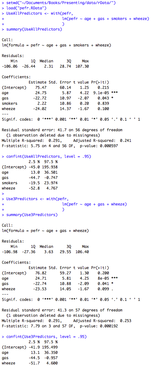
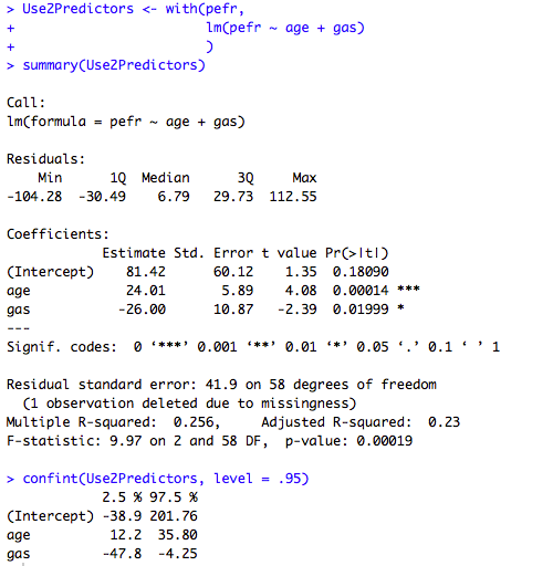
Figure 10.2 and Box 10.5 Code
Click here to show code with commentssetwd("~/Documents/Books/Presenting/data/rData/") load("pefr.RData") # Make a linear model object from a multiple regression with 4 predictors UseAllPredictors <- with(pefr, lm(pefr ~ age + gas + smokers + wheeze) ) summary(UseAllPredictors) # Show parameter estimates, p-values and model stats. # The confint() function can be use to print 95% CLs on the model coefficients # from a lm object. confint(UseAllPredictors, level = .95) # Show confidence intervals. # Instead of typing the model again you can update it. The update() function # expects a model for the first argument and a formula for the second. The # formula typically includes . ~ . to indicate the original outcome and the # original predictors model and then a + or a - to indicate the addition or # removal of predictors. # Use3Predictors <- update(UseAllPredictors, # the model to update # . ~ . - smokers # remove smokers # # Make a linear model object from a multiple regression with 3 predictors. Use3Predictors <- with(pefr, lm(pefr ~ age + gas + wheeze) ) summary(Use3Predictors) confint(Use3Predictors, level = .95) # Make a linear model object from a multiple regression with 2 predictors. Use2Predictors <- with(pefr, lm(pefr ~ age + gas) ) summary(Use2Predictors) confint(Use2Predictors, level = .95)
Figure 10.3 Output from multiple regression with categorical predictor variables
Box 10.8 Presentation of multiple regression with categorical predictor variable
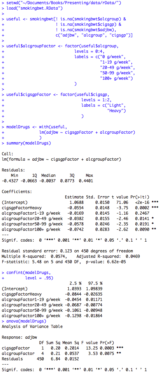
Box 10.8 and Figure 10.3 Code
Click here to show code with commentssetwd("~/Documents/Books/Presenting/data/rData/") load("smokingbwt.RData") # Make a data frame with no missing data on 3 analysis variables. useful <- smokingbwt[! is.na(smokingbwt$alcgroup) & # not missing ! is.na(smokingbwt$cigsgp) & ! is.na(smokingbwt$adjbw), # notice the , c("adjbw", "alcgroup", "cigsgp")] # keep 3 variables # Use the factor() function to make a variable in the useful data frame holding # a categorical factor version of the alcohol groups. See chapters 2 and 5 for more # details on factor(). useful$alcgroupFactor <- factor(useful$alcgroup, levels = 0:4, labels = c("0 g/week", "1-19 g/week", "20-49 g/week", "50-99 g/week", "100+ g/week") ) # Make a factor version of cigarette use. useful$cigsgpFactor <- factor(useful$cigsgp, levels = 1:2, labels = c("Light", "Heavy") ) # Make a linear model using the useful dataset where adjbw is predicted with # the two factors. modelDrugs <- with(useful, lm(adjbw ~ cigsgpFactor + alcgroupFactor) ) summary(modelDrugs) # Show the parameter estimates, p-values and model stats. confint(modelDrugs, # Show confidence intervals. level = .95) anova(modelDrugs) # Show overall p-values for factors.
Figure 10.5 Output for logistic regression
Box 10.12 Presenting the results for logistic regression
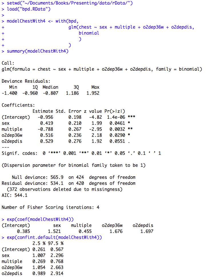
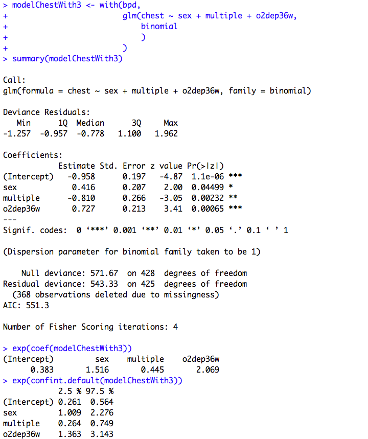
Figure 10.5 and Box 10.12 Code
Click here to show code with commentssetwd("~/Documents/Books/Presenting/data/rData/") load("bpd.RData") # Fit a logistic regression model. Save it as the object called modelChestWith4. modelChestWith4 <- with(bpd, # The glm() function fits generalized linear models. # Here it is used with the binomial family for logistic # regression. glm(chest ~ sex + multiple + o2dep36w + o2depdis, binomial # The default link will be logit. ) ) summary(modelChestWith4) # Show betas with P-values. # The exp() function calculates the exponential function. exp(coef(modelChestWith4)) # This exponentiates the coefficents to # get odds ratios. exp(confint.default(modelChestWith4)) # Get wald CLs on the ORs. modelChestWith3 <- with(bpd, glm(chest ~ sex + multiple + o2dep36w, binomial ) ) summary(modelChestWith3) exp(coef(modelChestWith3)) exp(confint.default(modelChestWith3))
Figure 10.6 Output for logistic regression with categorical predictor variables
Box 10.14 Presenting logistic regression with categorical predictor variables
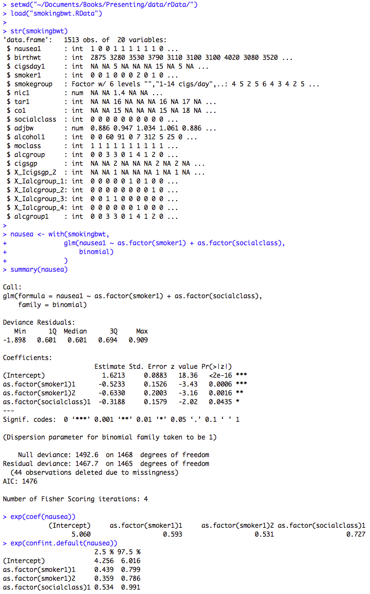
Figure 10.6 and Box 10.14 Code
Click here to show code with commentssetwd("~/Documents/Books/Presenting/data/rData/") load("smokingbwt.RData") # The str() function shows the structure of an object. It is useful to quickly # check to see if R will treat a variable as a numeric or categorical variable # when it makes models. str(smokingbwt) # Fit a logistic regression model and save it as the object called nausea. nausea <- with(smokingbwt, # This is a generalized linear model using the binomial family # and the logit link. Predict nausea with smoker1 and # socialclass as categorical factors. glm(nausea1 ~ as.factor(smoker1) + as.factor(socialclass), binomial) ) summary(nausea) # Show betas, p-values and model summary. exp(coef(nausea)) # Odds ratios are betas exponentiated. exp(confint.default(nausea)) # Make Wald CLs on the odds ratios.
Box 10.15 Presenting unadjusted and adjusted logistic regression
