Chapter 10: Multifactorial analyses using SAS
Figure 10.1 (a) Output for one-way analysis of variance
Box 10.3 Presenting the results for one-way analysis of variance
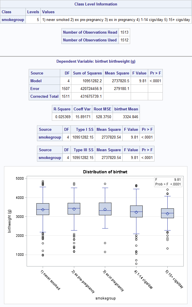
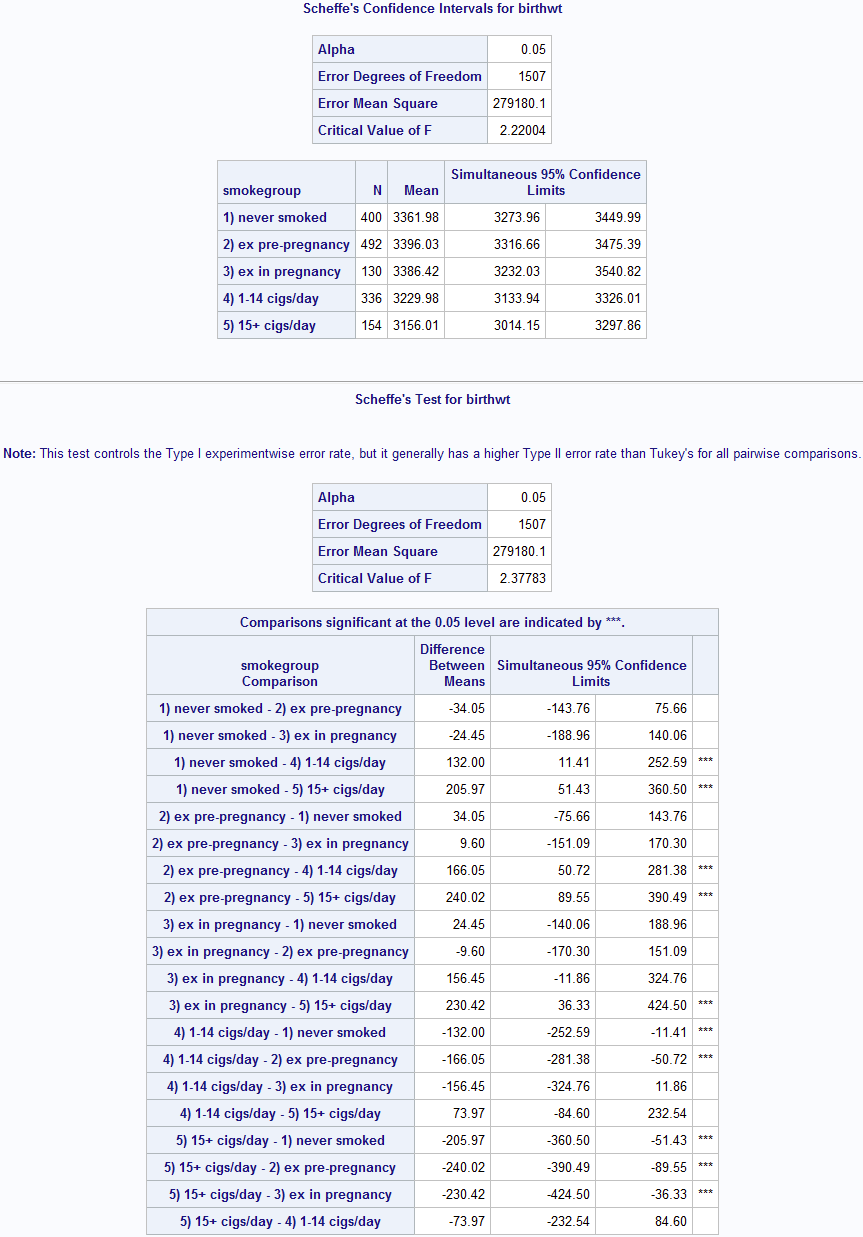
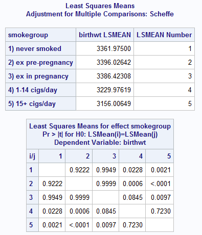
Figure 10.1 and Box 10.3 Code
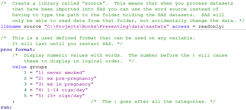
 Click here to show code as text
/*  Create a library called "source".  This means that when you process datasets
    that have been imported into SAS you can use the word source instead of
    having to type the path to the folder holding the SAS datasets.  SAS will
    only be able to read data from that folder, not accidentally change the data. */
libname source "C:\Projects\Books\Presenting\data\sasData" access = readonly;

/*  This is a user defined format that can be used on any variable.
    It will last until you restart SAS. */
proc format;
    /*  Display numeric values with words.  The number before the ) will cause
        these to display in logical order.  */
    value groups
        1 = "1) never smoked"
        2 = "2) ex pre-pregnancy"
        3 = "3) ex in pregnancy"
        4 = "4) 1-14 cigs/day"
        5 = "5) 15+ cigs/day"
    ;                          /*  The ; goes after all the categories. */
run;


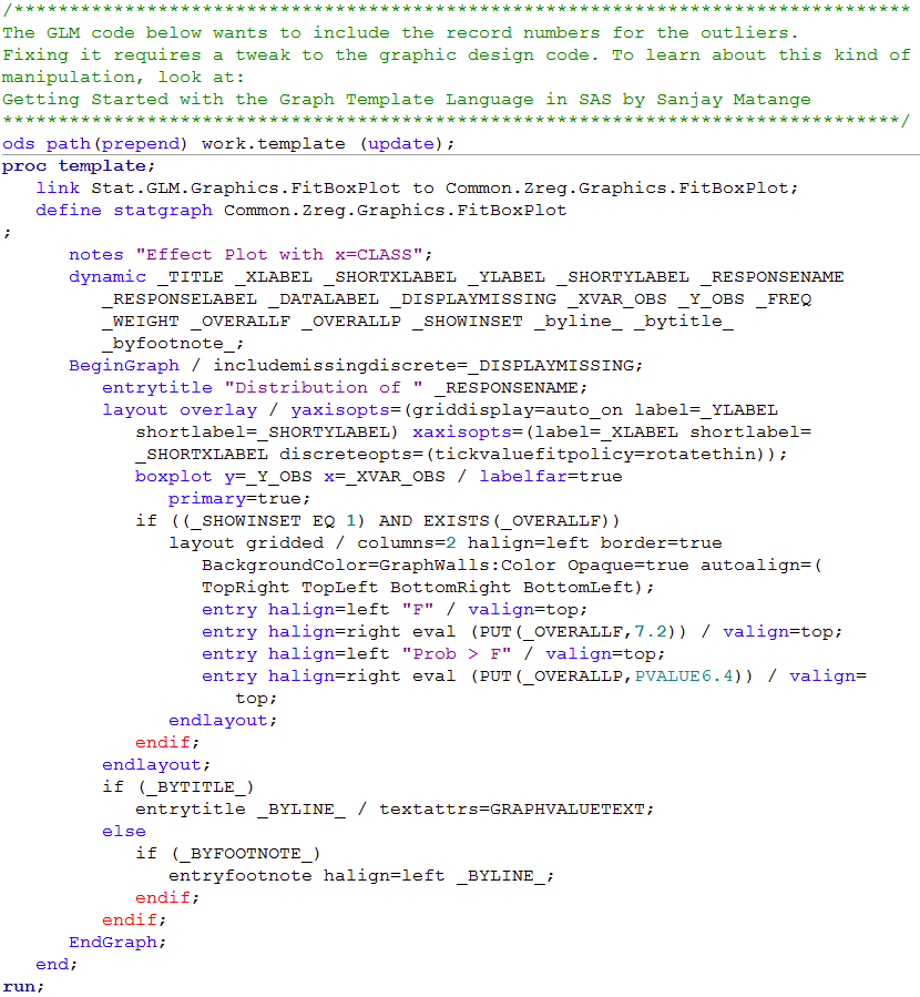
/*********************************************************************************
The GLM code below wants to include the record numbers for the outliers.
Fixing it requires a tweak to the graphic design code. To learn about this kind of
manipulation, look at:
Getting Started with the Graph Template Language in SAS by Sanjay Matange
*********************************************************************************/
ods path(prepend) work.template (update);
proc template;
   link Stat.GLM.Graphics.FitBoxPlot to Common.Zreg.Graphics.FitBoxPlot;
   define statgraph Common.Zreg.Graphics.FitBoxPlot
;
      notes "Effect Plot with x=CLASS";
      dynamic _TITLE _XLABEL _SHORTXLABEL _YLABEL _SHORTYLABEL _RESPONSENAME
         _RESPONSELABEL _DATALABEL _DISPLAYMISSING _XVAR_OBS _Y_OBS _FREQ
         _WEIGHT _OVERALLF _OVERALLP _SHOWINSET _byline_ _bytitle_
         _byfootnote_;
      BeginGraph / includemissingdiscrete=_DISPLAYMISSING;
         entrytitle "Distribution of " _RESPONSENAME;
         layout overlay / yaxisopts=(griddisplay=auto_on label=_YLABEL
            shortlabel=_SHORTYLABEL) xaxisopts=(label=_XLABEL shortlabel=
            _SHORTXLABEL discreteopts=(tickvaluefitpolicy=rotatethin));
            boxplot y=_Y_OBS x=_XVAR_OBS / labelfar=true
               primary=true;
            if ((_SHOWINSET EQ 1) AND EXISTS(_OVERALLF))
               layout gridded / columns=2 halign=left border=true
                  BackgroundColor=GraphWalls:Color Opaque=true autoalign=(
                  TopRight TopLeft BottomRight BottomLeft);
                  entry halign=left "F" / valign=top;
                  entry halign=right eval (PUT(_OVERALLF,7.2)) / valign=top;
                  entry halign=left "Prob > F" / valign=top;
                  entry halign=right eval (PUT(_OVERALLP,PVALUE6.4)) / valign=
                     top;
               endlayout;
            endif;
         endlayout;
         if (_BYTITLE_)
            entrytitle _BYLINE_ / textattrs=GRAPHVALUETEXT;
         else
            if (_BYFOOTNOTE_)
               entryfootnote halign=left _BYLINE_;
            endif;
         endif;
      EndGraph;
   end;
run;


proc template;
   define statgraph Stat.GLM.Graphics.BoxPlot ;
      dynamic _DEPVAR _CLASSVAR _GROUPDFBY _SHORTYLABEL _SHORTCLABEL _OVERALLF
         _OVERALLP _byline_ _bytitle_ _byfootnote_;
      BeginGraph;
         entrytitle "Distribution of " _DEPVAR;
         layout overlay / yaxisopts=(display=all gridDisplay=auto_on
            shortlabel=_SHORTYLABEL) xaxisopts=(shortlabel=_SHORTCLABEL
            discreteopts=(tickvaluefitpolicy=rotatethin));
            boxplot y=_DEPEN x=_GROUPDFBY / freq=_FREQ
               labelfar=on;
            layout gridded / columns=2 halign=left border=true BackgroundColor
               =GraphWalls:Color Opaque=true autoalign=(TopRight TopLeft
               BottomRight BottomLeft Right Left Top Bottom Center);
               entry halign=left "F" / valign=top;
               entry halign=right eval (PUT(_OVERALLF,7.2)) / valign=top;
               entry halign=left "Prob > F" / valign=top;
               entry halign=right eval (PUT(_OVERALLP,PVALUE6.4)) / valign=top
;
            endlayout;
         endlayout;
         if (_BYTITLE_)
            entrytitle _BYLINE_ / textattrs=GRAPHVALUETEXT;
         else
            if (_BYFOOTNOTE_)
               entryfootnote halign=left _BYLINE_;
            endif;
         endif;
      EndGraph;
   end;
run;

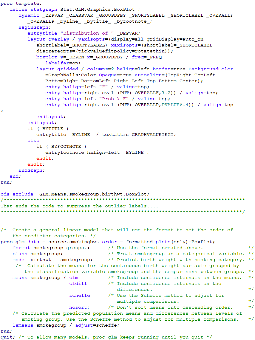
ods exclude  GLM.Means.smokegroup.birthwt.BoxPlot;
/*********************************************************************************
That ends the code to suppress the outlier labels....
*********************************************************************************/


/*  Create a general linear model that will use the format to set the order of
    the predictor categories. */
proc glm data = source.smokingbwt order = formatted plots(only)=BoxPlot;
    format smokegroup groups.;      /* Use the format created above.               */
    class smokegroup;               /* Treat smokegroup as a categorical variable. */
    model birthwt = smokegroup;     /* Predict birth weight with smoking category. */
     /*  Calculate the means for the continuous birth weight variable grouped by
        the classification variable smokegroup and the comparisons between groups. */
    means smokegroup / clm          /* Include confidence intervals on the means.  */
                       cldiff       /* Include confidence intervals on the
                                       differences.                                */
                       scheffe      /* Use the Scheffe method to adjust for
                                       multiple comparisons.                       */
                       nosort;      /* Don't sort means into descending order.     */
    /* Calculate the predicted population means and differences between levels of
       smoking group. Use the Scheffe method to adjust for multiple comparisons.   */
    lsmeans smokegroup / adjust=scheffe;
run;
quit; /* To allow many models, proc glm keeps running until you quit */
Figure 10.2 Output for multiple regression
Box 10.5 Presenting the results of multiple regression

Figure 10.2 and Box 10.5 Code
 Click here to show code as text
libname source "C:\Projects\Books\Presenting\data\sasData" access = readonly;

proc reg data = source.pefr ;
    /*  Predict pefr and include confidence limits on the parameter estimates (betas).
        The text before the : is an optional label on the model. */
    UseAllPredictors: model pefr = age gas smokers wheeze / clb;
    Use3Predictors:   model pefr = age gas wheeze / clb;
    Use2predictors:   model pefr = age gas / clb;
run;
quit; /* To allow many models, reg keeps running until you quit. */
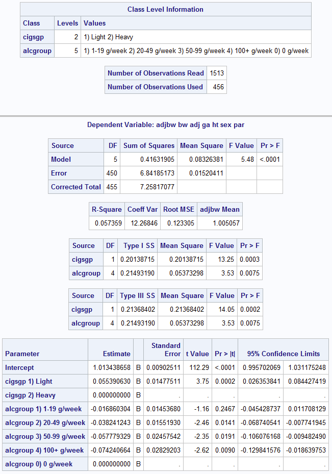
Figure 10.3 Output from multiple regression with categorical predictor variables
Box 10.8 Presentation of multiple regression with categorical predictor variable
Box 10.8 Figure 10.3 Code
 Click here to show code as text
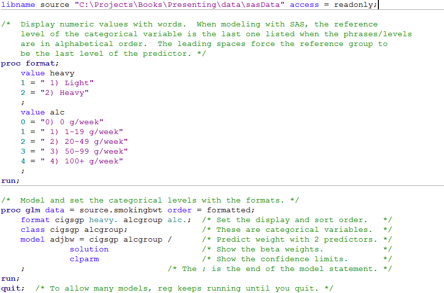
libname source "C:\Projects\Books\Presenting\data\sasData" access = readonly;

/*  Display numeric values with words.  When modeling with SAS, the reference
    level of the categorical variable is the last one listed when the phrases/levels
    are in alphabetical order.  The leading spaces force the reference group to
    be the last level of the predictor. */
proc format;
    value heavy
    1 = " 1) Light"
    2 = "2) Heavy"
    ;
    value alc
    0 = "0) 0 g/week"
    1 = " 1) 1-19 g/week"
    2 = " 2) 20-49 g/week"
    3 = " 3) 50-99 g/week"
    4 = " 4) 100+ g/week"
    ;
run;

/*  Model and set the categorical levels with the formats. */
proc glm data = source.smokingbwt order = formatted;
    format cigsgp heavy. alcgroup alc.;  /* Set the display and sort order.   */
    class cigsgp alcgroup;               /* These are categorical variables.  */
    model adjbw = cigsgp alcgroup /      /* Predict weight with 2 predictors. */
              solution                   /* Show the beta weights.            */
              clparm                     /* Show the confidence limits.       */
    ;                             /* The ; is the end of the model statement. */
run;
quit;  /* To allow many models, reg keeps running until you quit. */
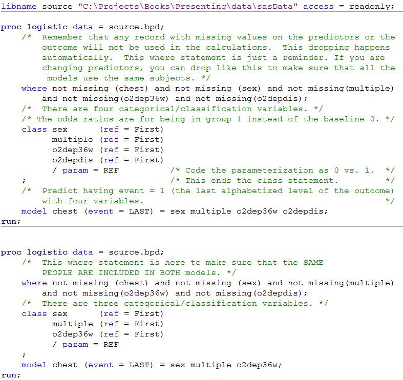
Figure 10.5 Output for logistic regression
Box 10.12 Presenting the results for logistic regression

Figure 10.5 Code
 Click here to show code as text
libname source "C:\Projects\Books\Presenting\data\sasData" access = readonly;

proc logistic data = source.bpd;
    /*  Remember that any record with missing values on the predictors or the
        outcome will not be used in the calculations.  This dropping happens
        automatically.  This where statement is just a reminder. If you are
        changing predictors, you can drop like this to make sure that all the
         models use the same subjects. */
    where not missing (chest) and not missing (sex) and not missing(multiple)
        and not missing(o2dep36w) and not missing(o2depdis);
    /*  There are four categorical/classification variables. */
    /* The odds ratios are for being in group 1 instead of the baseline 0. */
    class sex      (ref = First)
          multiple (ref = First)
          o2dep36w (ref = First)
          o2depdis (ref = First)
          / param = REF          /* Code the parameterization as 0 vs. 1.  */
    ;                            /* This ends the class statement.         */
    /*  Predict having event = 1 (the last alphabetized level of the outcome)
        with four variables.                                               */
    model chest (event = LAST) = sex multiple o2dep36w o2depdis;
run;


proc logistic data = source.bpd;
    /*  This where statement is here to make sure that the SAME
        PEOPLE ARE INCLUDED IN BOTH models. */
    where not missing (chest) and not missing (sex) and not missing(multiple)
        and not missing(o2dep36w) and not missing(o2depdis);
    /*  There are three categorical/classification variables. */
    class sex      (ref = First)
          multiple (ref = First)
          o2dep36w (ref = First)
          / param = REF
    ;
    model chest (event = LAST) = sex multiple o2dep36w;
run;
Figure 10.6 Output for logistic regression with categorical predictor variables
Box 10.14 Presenting logistic regression with categorical predictor variables
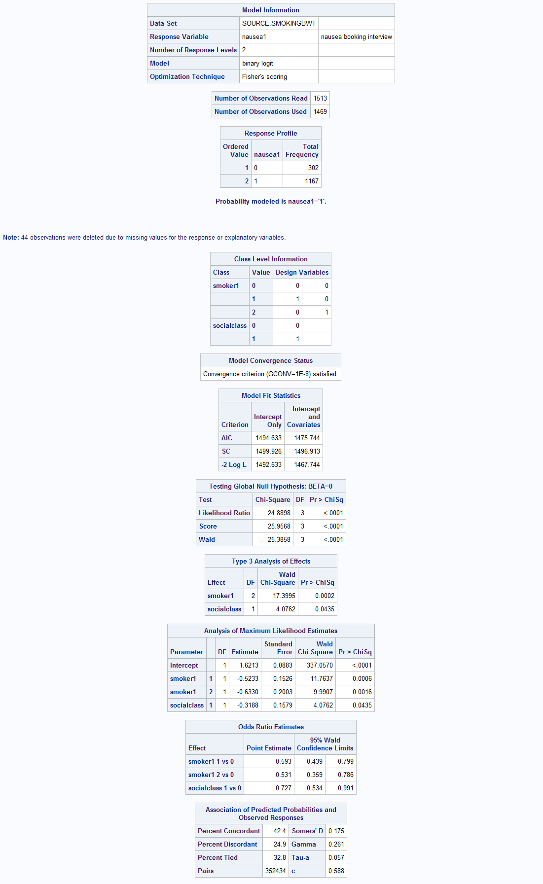
Figure 10.6 and Box 10.14 Code
 Click here to show code as text
libname source "C:\Projects\Books\Presenting\data\sasData" access = readonly;

proc logistic data = source.smokingbwt;
    /* There is no where statemen,t so the output notes who is dropped. */
    class smoker1 (ref = First)
          socialclass (ref = First)
          / param = ref
    ;
    model nausea1 (event = LAST) = smoker1 socialclass;
run;
Box 10.15 Presenting unadjusted and adjusted logistic regression

Box 10.15
 SAS can not easily produce this output.
code will be here.