Chapter 11: Survival analysis using R
Figure 11.1, Kaplan–Meier curve
Figure 11.2 Kaplan–Meier curve with logrank test
Figure 11.4 Output for Kaplan–Meier estimates of survival and logrank test
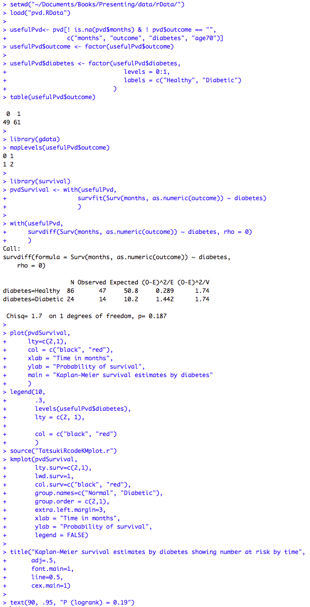
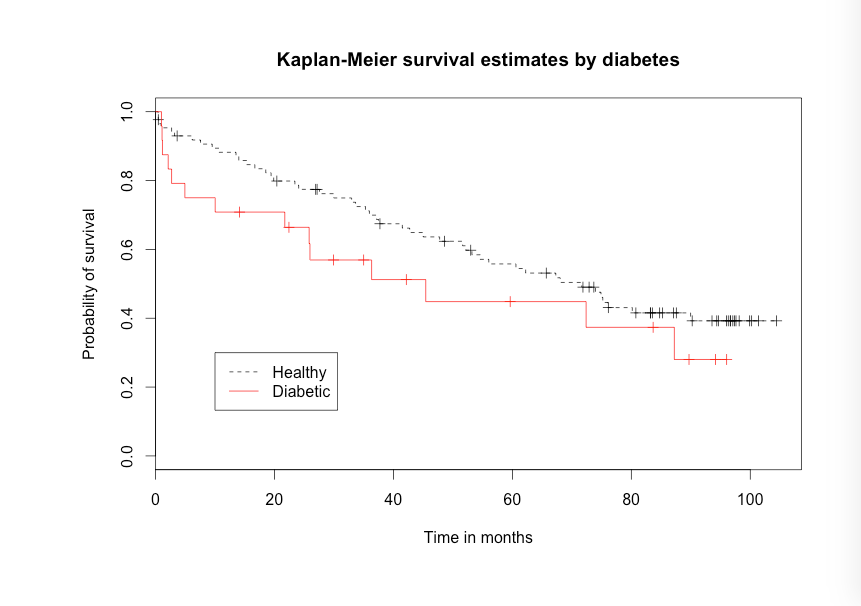
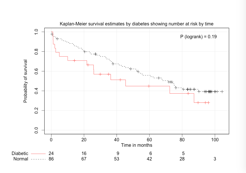
Figure 11.1, 11.2 and 11.4 Code
Click here to show code with comments# Tell R where you will be working. R will look here for your data: setwd("~/Documents/Books/Presenting/data/rData/") # See chapter 2 for more details on the setwd() function. # Use the load() function to load the dataset pvd.RData out of the current # folder/directory into R's interactive working memory/environment. See chapter # 2 for more details. load("pvd.RData") # The code shows how to make a data frame that keeps the 4 variables of interest # for the records/observations where the month variable is not missing and the # outcome is not blank. The logic checks inside of the [ ] generate # values indicating which rows and columns to include in the new data frame. # Read the syntax as: [ row check , column check ]. Remember that # R uses == to check for equality and ! means "not". ! changes true into false # and it changes false into true. The is.na() function checks for missing # values and returns a vector of true and false values. usefulPvd<- pvd[! is.na(pvd$months) & ! pvd$outcome == "", # rows to keep , c("months", "outcome", "diabetes", "age70")] # columns to keep # The c() function used above can glue together a set of similar things, # in this case, a bunch of character stings, to make a vector. # The factor() function can be used to remake a categorical factor variable # without the blank level. See chapters 2 and 5 for more information on the # factor() function. usefulPvd$outcome <- factor(usefulPvd$outcome) usefulPvd$diabetes <- factor(usefulPvd$diabetes, levels = 0:1, labels = c("Healthy", "Diabetic") ) # The table() function does simple cross tabulation tables. table(usefulPvd$outcome) # Count the alive and the dead people. # Load the survival package for survfit() and survdiff() functions. library(survival) pvdSurvival <- with(usefulPvd, # Predict number of months of survival with diabetes. # The as.numeric() function coerces the outcome variable to be # numeric if it is not already numeric(outcome). # The survfit() function makes a survfit object with details # on a Cox model. It can be used to show median survival # information by typing the object name or it can print a # survival curve when used with plot, for example, # plot(pvdSurvival) # The Surv() function makes an object that has information # on the outcome/survival. It is typically used like this # with the survfit() function. survfit(Surv(months, as.numeric(outcome)) ~ diabetes) ) with(usefulPvd, # Predict number of months of survival with diabetes. The survdiff() function # with rho = 0 does a log-rank test to compare the survival in the # predictor factor diabetes. survdiff(Surv(months, as.numeric(outcome)) ~ diabetes, rho = 0) ) # Use the plot() function to draw the KM curve. Because the object it is drawing # is a "survfit" object, it draws the KM curve. plot(pvdSurvival, # survival plot using model from above lty=c(2,1), # solid line, dotted line col = c("black", "red"), # first line red xlab = "Time in months", # label x-axis ylab = "Probability of survival", main = "Kaplan-Meier survival estimates by diabetes" ) # The legend() function adds a legend to an existing plot created using the plot() # function. You can set many options. Type ?par to see options like the line # type (lty) or the line colors (col). legend(10, # legend at x-axis position 10 .3, # legend at y-axis position .3 # The levels() function can be used to get the factor labels for a # variable. levels(usefulPvd$diabetes), # the values that are in the key lty = c(2, 1), # Specify a dashed and solid line for the # key. col = c("black", "red") ) # A user-written function that produces a graphic, including the number left at # risk, can be found here: # http://biostat.mc.vanderbilt.edu/wiki/Main/TatsukiRcode # If you save it as an r file called TatsukiRcodeKMplot.r in your working # directory, then the source() function will include it when you run your code. source("TatsukiRcodeKMplot.r") kmplot(pvdSurvival, lty.surv=c(2,1), # dashed, solid lines lwd.surv=1, # width of curves col.surv=c("black", "red"), # color of curves group.names=c("Normal", "Diabetic"), # labels group.order = c(2,1), # normal above diabetic extra.left.margin=3, # leave room for labels xlab = "Time in months", # label x-axis ylab = "Probability of survival", # label y-axis legend = FALSE) # no legend in body of picture # The title() function can add titles to many common plots including graphics # created by the plot(). To learn more look here: # http://www.statmethods.net/advgraphs/axes.html title("Kaplan-Meier survival estimates by diabetes showing number at risk by time", adj=.5, # centered (default) font.main=1, # which font line=0.5, # distance from plot cex.main=1) # size of font # The text() function can be used to add annotation to plots produced by the # plot() function. The first argument gives the x-axis location, the second # is used for the y-axis and the third is the text that is added to the plot. text(90, .95, "P (logrank) = 0.19") # Center extra text at (90, .95)
Figure 11.3
The data for this graphic are not available.
Figure 11.5 Output for Cox regression with one predictor available
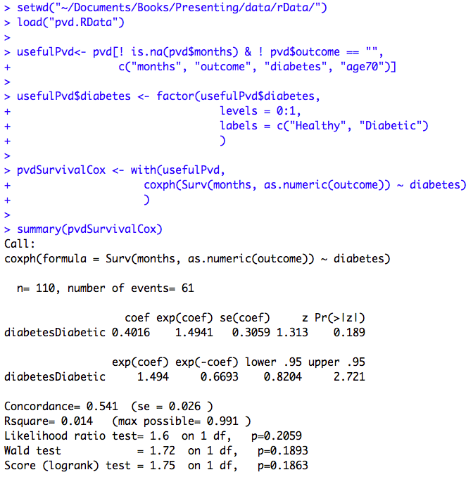
Figure 11.5 Code
Click here to show code with commentssetwd("~/Documents/Books/Presenting/data/rData/") load("pvd.RData") usefulPvd$diabetes <- factor(usefulPvd$diabetes, levels = 0:1, labels = c("Healthy", "Diabetic") ) pvdSurvivalCox <- with(usefulPvd, # The coxph() function fits a cox proportional hazards model. coxph(Surv(months, as.numeric(outcome)) ~ hasDiabetes) ) # The summary() function pays attention to the type of object it is summarizing. # Here, because the object class is coxph, it gives the model, the coefficients, # and several statistics. See chapters 2 and 9 for more details. summary(pvdSurvivalCox) # Display the Cox model.
Figure 11.6 Output for Cox regression with more than one predictor variable
Box 11.8 Presenting Cox regression analysis
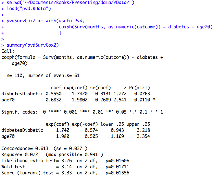
Figure 11.6 and Box 11.8 Code
Click here to show code with commentssetwd("~/Documents/Books/Presenting/data/rData/") load("pvd.RData") pvdSurvCox2 <- with(usefulPvd, # Predict number of months of survival with diabetes and # age > 70 indicator. Notice that the Surv() function # call is on the left side of the ~ which indicates that # it is the outcome of the model. coxph(Surv(months, as.numeric(outcome)) ~ diabetes + age70) ) summary(pvdSurvCox2) # Display the Cox model.