Home > Output
Chapter 2: Introducton to the research process using STATA
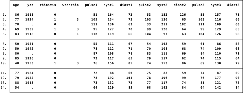
Figure 2.1 and Figure 2.3

Figure 2.1 Portion of a dataset showing data collected for particiapnts in a screening survey (example)

Figure 2.3 Checking for errors in the data (example)
Figure 2.1 and Figure 2.3 Code

Click here to show code as text
// load the rhinitis data
use "C:\Projects\Books\Presenting\data\stataData\rhinitis.dta", clear

/*****************************/
/* Figure 2.1 and Figure 2.3 */
/*****************************/

// display the first 14 records
list in 1/14
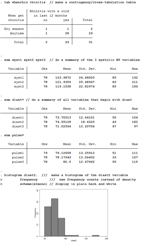
Figure 2.4

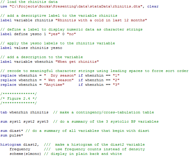
Figure 2.4 Code

Click here to show code as text
// load the rhinitis data
use "C:\Projects\Books\Presenting\data\stataData\rhinitis.dta", clear

// add a descriptive label to the variable rhinitis
label variable rhinitis "Rhinitis with a cold in last 12 months"

// define a label to display numeric data as character strings
label define yesno 1 "yes" 0 "no"

// apply the yesno labels to the rhinitis variable
label values rhinitis yesno

// add a description to the variable
label variable whenrhin "When get rhinitis"

// recode to meaningful character strings using leading spaces to force sort order
replace whenrhin = "  Dry season" if whenrhin == "1"
replace whenrhin = " Wet season"  if whenrhin == "2"
replace whenrhin = "Anytime"      if whenrhin == "3"

/**************/
/* Figure 2.4 */
/**************/

tab whenrhin rhinitis  // make a contingency/cross-tabulation table

sum syst1 syst2 syst3  // do a summary of the 3 systolic BP variables

sum diast* // do a summary of all variables that begin with diast
sum pulse*

histogram diast2,  ///  make a histogram of the diast2 variable
	frequency      ///  use frequency counts instead of density
	scheme(s1mono) // display in plain back and white

