Home > Output
Chapter 5: Introduction to presenting statistical analyses using STATA
Box 5.3 Assessing non-response bias

Box 5.3 Code

Click here to show code as text
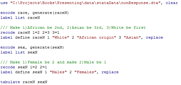
use "C:\Projects\Books\Presenting\data\stataData\nonResponse.dta", clear

encode race, generate(raceN)
label list raceN

/// Make 1)African be 2nd, 2)Asian be 3rd, 3)White be first
recode raceN 1=2 2=3 3=1
label define raceN 1 "White" 2 "African origin" 3 "Asian", replace

encode sex, generate(sexN)
label list sexN

/// Make 1)Female be 2 and make 2)Male be 1
recode sexN 1=2 2=1
label define sexN 1 "Males" 2 "Females", replace

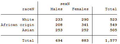
tabulate raceN sexN
Box 5.4 Population profile from a report


Box 5.4 Code

Click here to show code as text
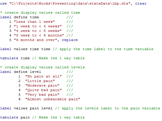
use "C:\Projects\Books\Presenting\data\stataData\lbp.dta", clear

* create display values called time
label define time            ///
	1 "Less than 1 week"     ///
	2 "1 week to < 4 weeks"  ///
	3 "4 week to < 8 weeks"  ///
	4 "8 week to < 6 months" ///
	5 "6 months and over", replace

label values time time // apply the time label to the time variable

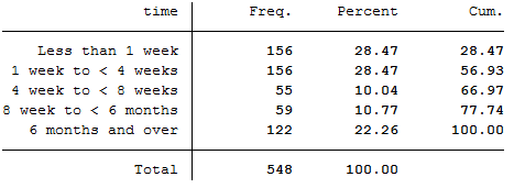
tabulate time // Make the 1 way table

* create display values called levels
label define level           ///
        1  "No pain at all"  ///
        2  "Little pain"     ///
        3  "Moderate pain"   ///
        4  "Quite bad pain"  ///
        5  "Very bad pain"   ///
        6  "Almost unbearable pain"

label values pain level // apply the levels label to the pain variable

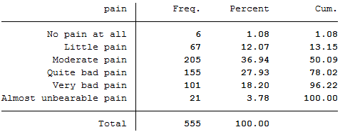
tabulate pain // Make the 1 way table
Table 5.1 Single Concise table from a paper with adjusted and unadjusted estimates
Table 5.2 Table suitable for an oral presentation
Examples of how to do these analyses come later in the book (e.g., Figure 7.11 shows how to do a Chi-Square test and calculate relative risk for data for age; figure 10.4 shows how to do adjusted analyses using logistic regression which gives odds ratios, estimating the estimating the adjusted relative risk.
Figure 5.5 Calculating the confidence interval of a geometric mean


Figure 5.5 Code

Click here to show code as text
use "C:\Projects\Books\Presenting\data\stataData\hdl.dta", clear
ci loghdl
means hdl
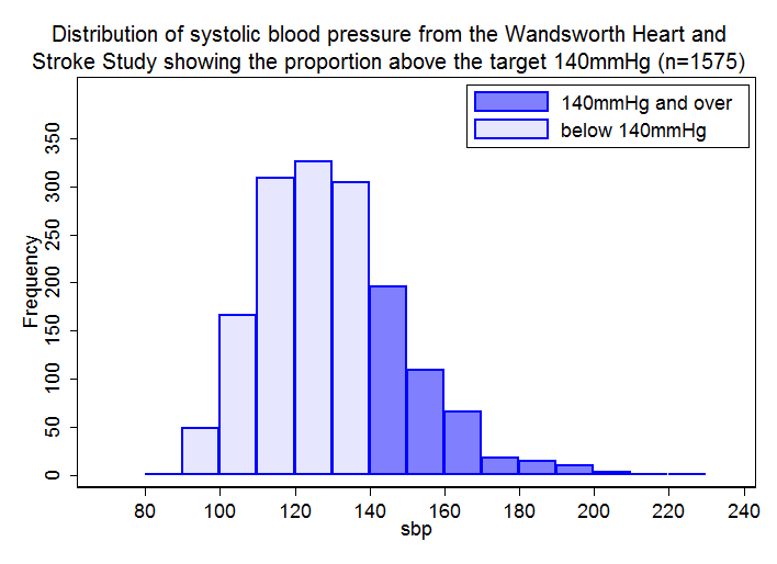
Figure 5.6

Figure 5.6 Code

Click here to show code as text
use "C:\Projects\Books\Presenting\data\stataData\whss.dta", clear

gen target=0 if sbp<140
replace target=1 if sbp>=140
replace target=. if sbp==.

twoway histogram sbp if target, freq  ///
title(Distribution of systolic blood pressure from the Wandsworth Heart and  ,span size(medium small)) ///
subtitle(Stroke Study showing the proportion above the target 140mmHg (n=1575), span size(medium small)) ///
start(70)  width(10) bcolor(blue*.5) blcolor(blue)  yscale(r(0 400)) xlabel(80 100 120 140 160 180 200 220 240) ylabel(0 50 100 150 200 250 300 350) || ///
histogram sbp if !target ,  freq   ///
start(70) width(10) bcolor(blue*.1) blcolor(blue)  ///
legend(order(1 "140mmHg and over" 2 "below 140mmHg") col(1) pos(1) ring(0))
