Chapter 6: Single group studies using R
Figure 6.1 Output for calculating a prevalence and 95% confidence interval
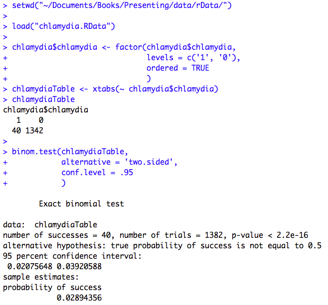
Figure 6.1 Code
Click here to show code with comments
# Tell R where you will be working. R will look here for your data: setwd("~/Documents/Books/Presenting/data/rData/") # See chapter 2 for more details on the setwd() funciton. # Use the load() function to load the dataset ghana.RData out of the current # folder/directory into R's interactive working memory/environment. See chapter # 2 for more details. load("chlamydia.RData") # The factor() function below makes sure the variable called chlamydia in # the chlamydia dataset is processed as a categorical factor variable. It has # the values 0 and 1. The code sets the values to display in the right order. # R functions use a comma-delimited set of details. Programmers call # the details that a function understands "arguments". Notice the ( following # the word factor and the commas ending the lines with the arguments until # the closing ) . chlamydia$chlamydia <- factor(chlamydia$chlamydia, # Use the chlamydia # variable in the # chlamydia data frame. levels = c('1', '0'), # There are two levels to # the variable. ordered = TRUE # Pay attention to the 1 # before 0 order. ) # The xtabs() function can be used to generate frequency count tables. # Usually the ~ is used when you are doing predictive modeling. Typically you # type the outcome/response variable on the left and the predictors on the # right. Here the code is just processing a categorical variable but not # doing meaningful modeling. chlamydiaTable <- xtabs(~ chlamydia$chlamydia) # Make a freq count table. chlamydiaTable # Show the freq count table. # Use the binom.test() function to request exact binomial confidence limits. binom.test(chlamydiaTable, alternative = 'two.sided', conf.level = .95 )
Figure 6.2 Calculating sensitivity and specificity
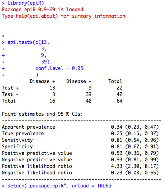
Figure 6.2 Code
Click here to show code with comments# The library() function attaches a package full of functions (and sometimes # data frames) to R's "search list". When you type epi.tests(), R searches that # list to figure out what to do. If you have not attached the package that # included a epi.tests() function, R will complain that it can not find the # function "epi.tests". # You can encounter problems when two packages include objects with the same # name. R will give a warning like: # The following object(s) are masked ... # when you attach a package that includes a function that is already in the # search list. R calls this problem masking. The detach() function, shown # below, can be used to remove packages from the search list and help avoid this # problem. # # Load the epiR package to have access to the epi.tests function. library(epiR) # The epi.tests() function gives estimates with exact confidence limits. It # expects a vector (what most people would call a list or set) of numbers for its # first argument. The c() function can glue together a set of similar things, # for example, a bunch of numbers, to make a vector. epi.tests(c(13, # number of obs where true disease status is positive and test is positive 3, # number of obs where true disease status is positive and test is negative 9, # number of obs where true disease status is negative and test is positive 39), # number of obs where true disease status is negative and test is positive conf.level = 0.95 ) detach("package:epiR", unload = TRUE) # prevent masking conflicts
Box 6.3 Screening study with a rare condition
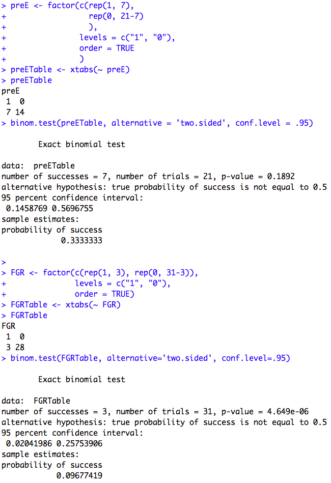
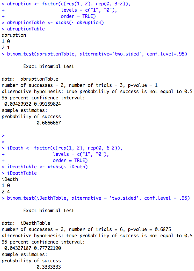
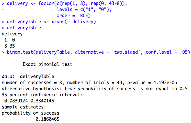
Box 6.3 Code
Click here to show code with comments# This creates the data and treats it as a categorical variable. The rep() # function repeats the first argument. The second argument has the count of # the repetitions. preE <- factor(c(rep(1, 7), rep(0, 21-7) ), levels = c("1", "0"), order = TRUE ) preETable <- xtabs(~ preE) preETable # Look at the table count. binom.test(preETable, alternative = 'two.sided', conf.level = .95) FGR <- factor(c(rep(1, 3), rep(0, 31-3)), levels = c("1", "0"), order = TRUE) FGRTable <- xtabs(~ FGR) FGRTable binom.test(FGRTable, alternative='two.sided', conf.level=.95) abruption <- factor(c(rep(1, 2), rep(0, 3-2)), levels = c("1", "0"), order = TRUE) abruptionTable <- xtabs(~ abruption) abruptionTable binom.test(abruptionTable, alternative='two.sided', conf.level=.95) iDeath <- factor(c(rep(1, 2), rep(0, 6-2)), levels = c("1", "0"), order = TRUE) iDeathTable <- xtabs(~ iDeath) iDeathTable binom.test(iDeathTable, alternative = 'two.sided', conf.level = .95) delivery <- factor(c(rep(1, 8), rep(0, 43-8)), levels = c("1", "0"), order = TRUE) deliveryTable <- xtabs(~ delivery) deliveryTable binom.test(deliveryTable, alternative = 'two.sided', conf.level = .95)