Chapter 7: Comparing two groups using SAS
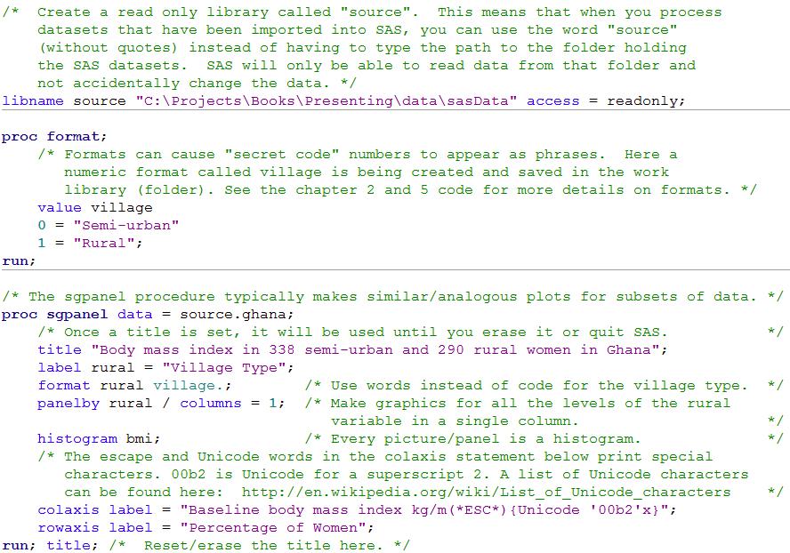
Figure 7.1 Histogram of two groups on one graph
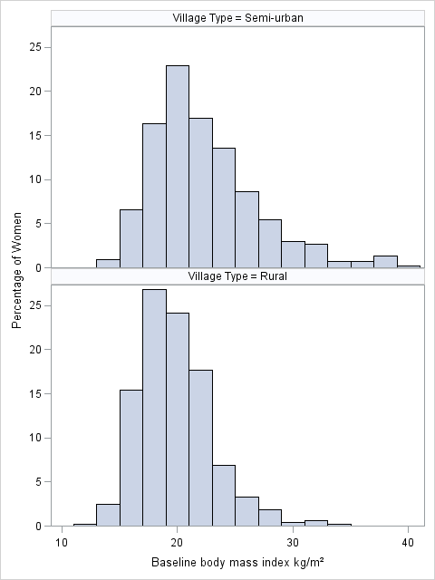
Figure 7.1 Code
 Click here to show code as text
/*  Create a read only library called "source".  This means that when you process
    datasets that have been imported into SAS, you can use the word "source"
    (without quotes) instead of having to type the path to the folder holding
    the SAS datasets.  SAS will only be able to read data from that folder and
    not accidentally change the data. */
libname source "C:\Projects\Books\Presenting\data\sasData" access = readonly;

proc format;
    /* Formats can cause "secret code" numbers to appear as phrases.  Here a
       numeric format called village is being created and saved in the work
       library (folder). See the chapter 2 and 5 code for more details on formats. */
    value village
    0 = "Semi-urban"
    1 = "Rural";
run;

/* The sgpanel procedure typically makes similar/analogous plots for subsets of data. */
proc sgpanel data = source.ghana;
    /* Once a title is set, it will be used until you erase it or quit SAS.           */
    title "Body mass index in 338 semi-urban and 290 rural women in Ghana";
    label rural = "Village Type";
    format rural village.;        /* Use words instead of code for the village type.  */
    panelby rural / columns = 1;  /* Make graphics for all the levels of the rural
                                     variable in a single column.                     */
    histogram bmi;                /* Every picture/panel is a histogram.              */
    /* The escape and Unicode words in the colaxis statement below print special
       characters. 00b2 is Unicode for a superscript 2. A list of Unicode characters
       can be found here:  http://en.wikipedia.org/wiki/List_of_Unicode_characters    */
    colaxis label = "Baseline body mass index kg/m(*ESC*){Unicode '00b2'x}";
    rowaxis label = "Percentage of Women";
run; title; /*  Reset/erase the title here. */
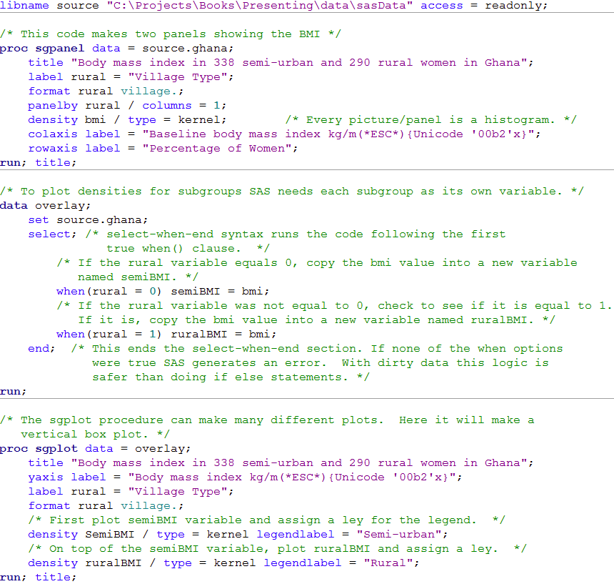
Figure 7.2 Two pannel or overlapping density plots for two groups
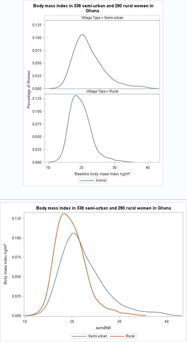
Figure 7.2 Code
 Click here to show code as text
libname source "C:\Projects\Books\Presenting\data\sasData" access = readonly;

/* This code makes two panels showing the BMI */
proc sgpanel data = source.ghana;
    title "Body mass index in 338 semi-urban and 290 rural women in Ghana";
    label rural = "Village Type";
    format rural village.;
    panelby rural / columns = 1;
    density bmi / type = kernel;        /* Every picture/panel is a histogram. */
    colaxis label = "Baseline body mass index kg/m(*ESC*){Unicode '00b2'x}";
    rowaxis label = "Percentage of Women";
run; title;

/* To plot densities for subgroups SAS needs each subgroup as its own variable. */
data overlay;
    set source.ghana;
    select; /* select-when-end syntax runs the code following the first
               true when() clause.  */
        /* If the rural variable equals 0, copy the bmi value into a new variable
           named semiBMI. */
        when(rural = 0) semiBMI = bmi;
        /* If the rural variable was not equal to 0, check to see if it is equal to 1.
           If it is, copy the bmi value into a new variable named ruralBMI. */
        when(rural = 1) ruralBMI = bmi;
    end;  /* This ends the select-when-end section. If none of the when options
             were true SAS generates an error.  With dirty data this logic is
             safer than doing if else statements. */
run;

/* The sgplot procedure can make many different plots.  Here it will make a
   vertical box plot. */
proc sgplot data = overlay;
    title "Body mass index in 338 semi-urban and 290 rural women in Ghana";
    yaxis label = "Body mass index kg/m(*ESC*){Unicode '00b2'x}";
    label rural = "Village Type";
    format rural village.;
    /* First plot semiBMI variable and assign a ley for the legend.  */
    density SemiBMI / type = kernel legendlabel = "Semi-urban";
    /* On top of the semiBMI variable, plot ruralBMI and assign a ley.  */
    density ruralBMI / type = kernel legendlabel = "Rural";
run; title;
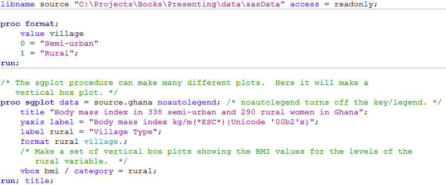
Figure 7.3 Box and whisker plot for a continuous variable in two groups
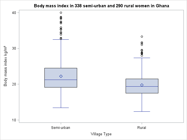
Figure 7.3 Code
 Click here to show code as text
libname source "C:\Projects\Books\Presenting\data\sasData" access = readonly;

proc format;
    value village
    0 = "Semi-urban"
    1 = "Rural";
run;

/* The sgplot procedure can make many different plots.  Here it will make a
   vertical box plot. */
proc sgplot data = source.ghana noautolegend; /* noautolegend turns off the key/legend. */
    title "Body mass index in 338 semi-urban and 290 rural women in Ghana";
    yaxis label = "Body mass index kg/m(*ESC*){Unicode '00b2'x}";
    label rural = "Village Type";
    format rural village.;
    /* Make a set of vertical box plots showing the BMI values for the levels of the
       rural variable.  */
    vbox bmi / category = rural;
run; title;
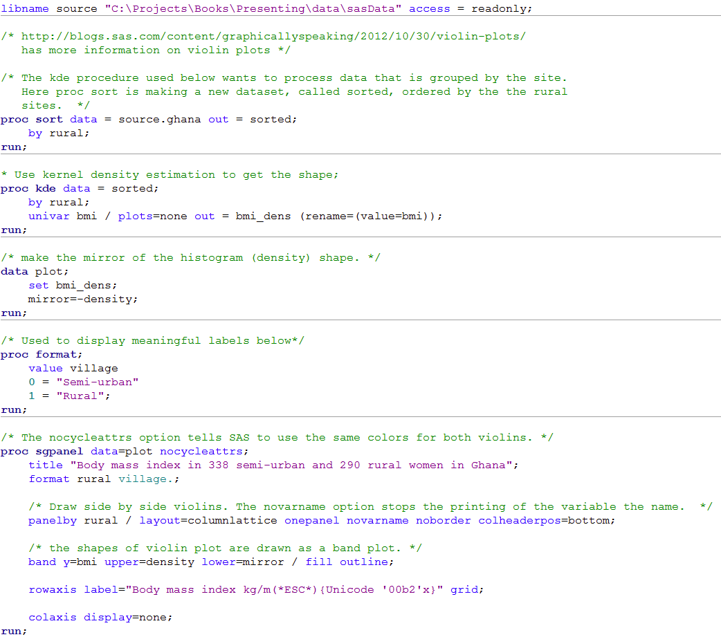
Figure 7.4 Violin plot for a continuous variable comparing two groups
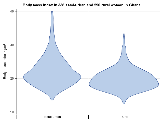
Figure 7.4 Code
 Click here to show code as text
libname source "C:\Projects\Books\Presenting\data\sasData" access = readonly;

/* http://blogs.sas.com/content/graphicallyspeaking/2012/10/30/violin-plots/
   has more information on violin plots */

/* The kde procedure used below wants to process data that is grouped by the site.
   Here proc sort is making a new dataset, called sorted, ordered by the the rural
   sites.  */
proc sort data = source.ghana out = sorted;
    by rural;
run;

* Use kernel density estimation to get the shape;
proc kde data = sorted;
    by rural;
    univar bmi / plots=none out = bmi_dens (rename=(value=bmi));
run;

/* make the mirror of the histogram (density) shape. */
data plot;
    set bmi_dens;
    mirror=-density;
run;

/* Used to display meaningful labels below*/
proc format;
	value village
	0 = "Semi-urban"
	1 = "Rural";
run;

/* The nocycleattrs option tells SAS to use the same colors for both violins. */
proc sgpanel data=plot nocycleattrs;
	title "Body mass index in 338 semi-urban and 290 rural women in Ghana";
    format rural village.;

    /* Draw side by side violins. The novarname option stops the printing of the variable the name.  */
    panelby rural / layout=columnlattice onepanel novarname noborder colheaderpos=bottom;

    /* the shapes of violin plot are drawn as a band plot. */
    band y=bmi upper=density lower=mirror / fill outline;

    rowaxis label="Body mass index kg/m(*ESC*){Unicode '00b2'x}" grid;

    colaxis display=none;
run;
Figure 7.5 Dot plot for a continuous variable comparing two groups
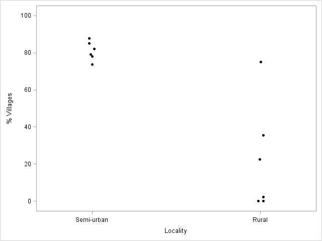
Figure 7.5 Code
 Click here to show code as text
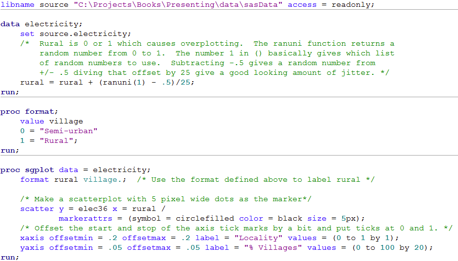
libname source "C:\Projects\Books\Presenting\data\sasData" access = readonly;

data electricity;
    set source.electricity;
    /*  Rural is 0 or 1 which causes overplotting.  The ranuni function returns a
        random number from 0 to 1.  The number 1 in () basically gives which list
        of random numbers to use.  Subtracting -.5 gives a random number from
        +/- .5 diving that offset by 25 give a good looking amount of jitter. */
    rural = rural + (ranuni(1) - .5)/25;
run;

proc format;
	value village
	0 = "Semi-urban"
	1 = "Rural";
run;

proc sgplot data = electricity;
    format rural village.;  /* Use the format defined above to label rural */

    /* Make a scatterplot with 5 pixel wide dots as the marker*/
	scatter y = elec36 x = rural /
			markerattrs = (symbol = circlefilled color = black size = 5px);
    /* Offset the start and stop of the axis tick marks by a bit and put ticks at 0 and 1. */
	xaxis offsetmin = .2 offsetmax = .2 label = "Locality" values = (0 to 1 by 1);
	yaxis offsetmin = .05 offsetmax = .05 label = "% Villages" values = (0 to 100 by 20);
run;
Figure 7.6 Histogram of a variable to check for normality
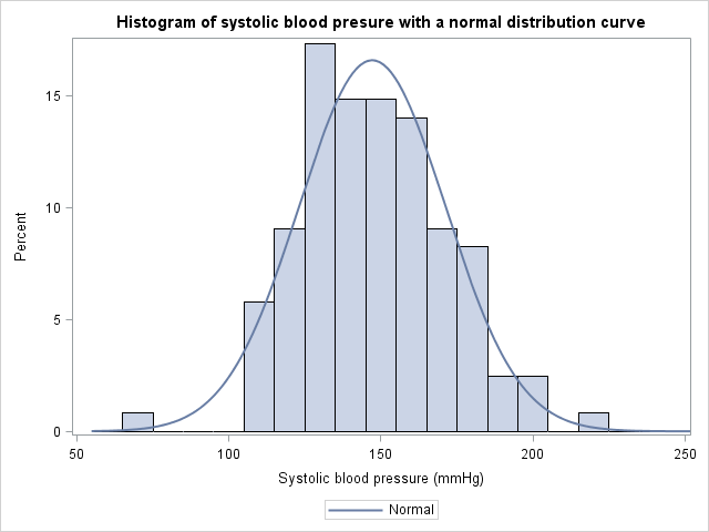
Figure 7.6 Code
 Click here to show code as text
libname source "C:\Projects\Books\Presenting\data\sasData" access = readonly;

proc sgplot data = source.pvd;
	title "Histogram of systolic blood pressure with a normal distribution curve";
	label sbp = "Systolic blood pressure (mm Hg)";
	histogram sbp / nbins = 25; /* nbins sets the number of bins/bar in the histogram */
	xaxis values = (50 to 250 by 50); /* values set the tick marks on the axis        */
	density sbp; /* This overlays a normal/Gausian curve on top of the histogram.     */
run; title;
Figure 7.7 Output for an unpaired t-test
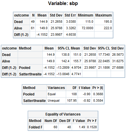
Figure 7.7 Code
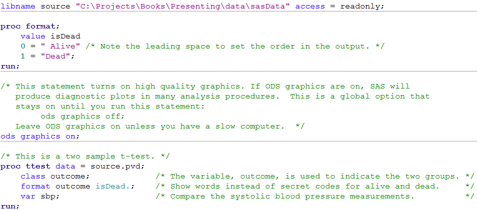 Click here to show code as text
libname source "C:\Projects\Books\Presenting\data\sasData" access = readonly;

proc format;
    value isDead
    0 = " Alive" /* Note the leading space to set the order in the output. */
    1 = "Dead";
run;

/* This statement turns on high quality graphics. If ODS graphics are on, SAS will
   produce diagnostic plots in many analysis procedures.  This is a global option that
   stays on until you run this statement:
        ods graphics off;
   Leave ODS graphics on unless you have a slow computer.  */
ods graphics on;

/* This is a two sample t-test. */
proc ttest data = source.pvd;
    class outcome;             /* The variable, outcome, is used to indicate the two groups. */
    format outcome isDead.;    /* Show words instead of secret codes for alive and dead.     */
    var sbp;                   /* Compare the systolic blood pressure measurements.          */
run;
Figure 7.8 Histograms of a skewed variable before and after log transformation
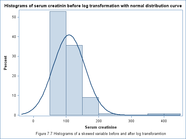
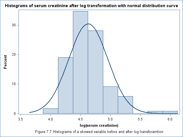
Figure 7.8 Code
 Click here to show code as text
libname source "C:\Projects\Books\Presenting\data\sasData" access = readonly;

proc sgplot data = source.pvd noautolegend;
    title "Histograms of serum creatinine before log transformation with normal distribution curve";
    label cr = "Serum creatinine";
    histogram cr;   /* First draw a histogram of Creatinine value. */
    density cr;     /* Next draw a density curve on top of the histogram. */
run; title;

proc sgplot data = source.pvd noautolegend;
    title "Histograms of serum creatinine after log transformation with normal distribution curve";
    label lcr = "log(serum creatinine)";
    histogram lcr;
    density lcr;
run; title;
Figure 7.9 Output for back transforming t-test data
Box 7.4 Presenting the findings of a t-test on log-transformed data
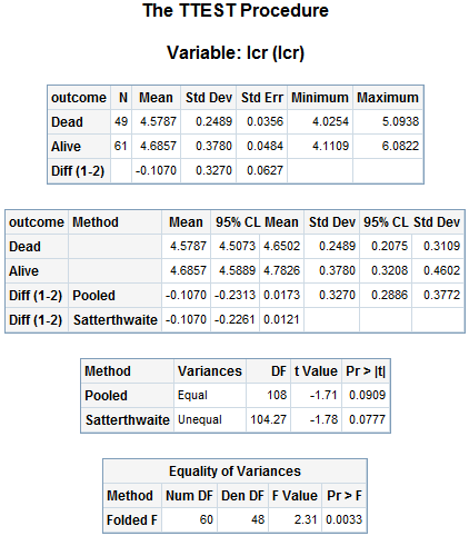
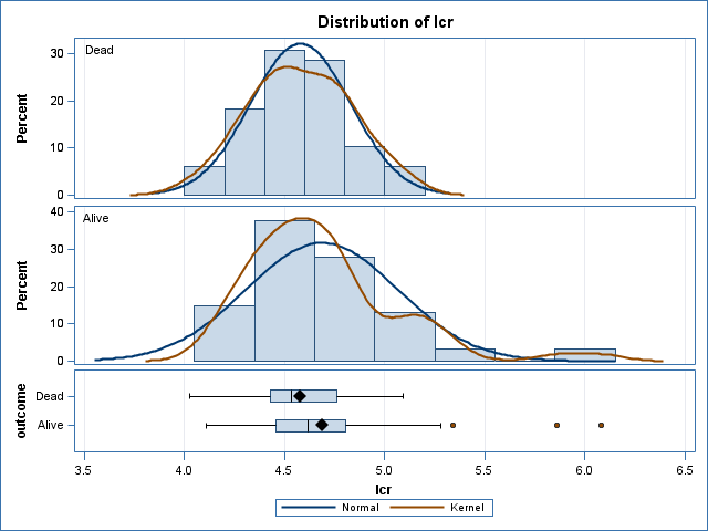
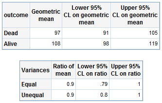
Figure 7.9 Code and Box 7.4
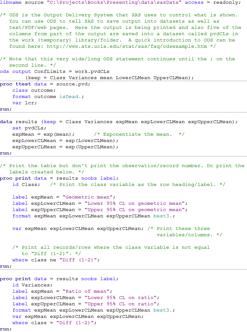 Click here to show code as text
libname source "C:\Projects\Books\Presenting\data\sasData" access = readonly;

/* ODS is the Output Delivery System that SAS uses to control what is shown.
   You can use ODS to tell SAS to save output into datasets as well as
   text/PDF/web pages.  Here the output is being printed and also five of the
   columns from part of the output are saved into a dataset called pvdCLs in
   the work (temporary) library/folder.  A quick introduction to ODS can be
   found here: http://www.ats.ucla.edu/stat/sas/faq/odsexample.htm */

/* Note that this very wide/long ODS statement continues until the ; on the
   second line. */
ods output ConfLimits = work.pvdCLs
        (keep = Class Variances mean LowerCLMean UpperCLMean);
proc ttest data = source.pvd;
    class outcome;
    format outcome isDead.;
    var lcr;
run;

data results (keep = Class Variances expMean expLowerCLMean expUpperCLMean);
    set pvdCLs;
    expMean = exp(mean);      /* Exponentiate the mean.  */
    expLowerCLMean = exp(LowerCLMean);
    expUpperCLMean = exp(UpperCLMean);
run;

/* Print the table but don't print the observation/record number. Do print the
   labels created below. */
proc print data = results noobs label;
    id Class;   /* Print the class variable as the row heading/label. */

    label expMean = "Geometric mean";
    label expLowerCLMean = "Lower 95% CL on geometric mean";
    label expUpperCLMean = "Upper 95% CL on geometric mean";
    format expMean expLowerCLMean expUpperCLMean best3.;

    var expMean expLowerCLMean expUpperCLMean; /* Print these three
                                                  variables/columns. */

    /* Print all records/rows where the class variable is not equal
       to "Diff (1-2)". */
    where class ne "Diff (1-2)";
run;

proc print data = results noobs label;
    id Variances;
    label expMean = "Ratio of mean";
    label expLowerCLMean = "Lower 95% CL on ratio";
    label expUpperCLMean = "Upper 95% CL on ratio";
    format expMean expLowerCLMean expUpperCLMean best3.;
    var expMean expLowerCLMean expUpperCLMean;
    where class = "Diff (1-2)";
run;
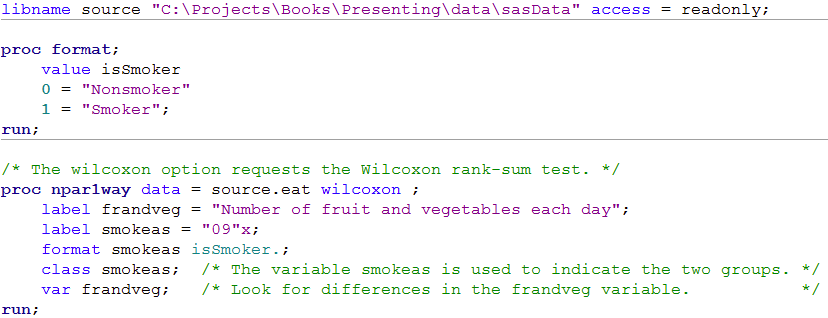
Figure 7.10 Table of data for and output from a Mann-Whitney U test
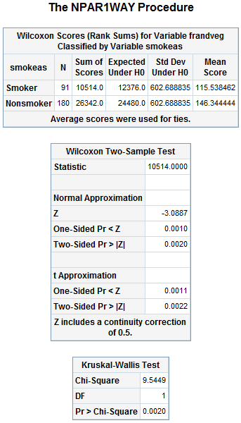
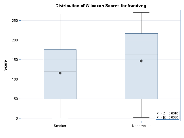
Figure 7.10 Code
 Click here to show code as text
libname source "C:\Projects\Books\Presenting\data\sasData" access = readonly;

proc format;
    value isSmoker
    0 = "Nonsmoker"
    1 = "Smoker";
run;

/* The wilcoxon option requests the Wilcoxon rank-sum test. */
proc npar1way data = source.eat wilcoxon ;
    label frandveg = "Number of fruit and vegetables each day";
    label smokeas = "09"x;
    format smokeas isSmoker.;
    class smokeas;  /* The variable smokeas is used to indicate the two groups. */
    var frandveg;   /* Look for differences in the frandveg variable.           */
run;
Figure 7.11 Output for chi-square test relative risk and risk difference
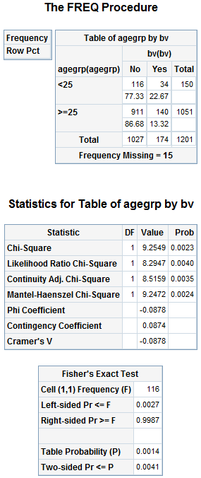
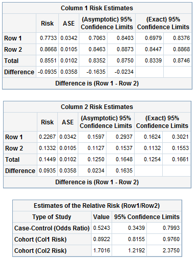
Figure 7.11 Code
 Click here to show code as text
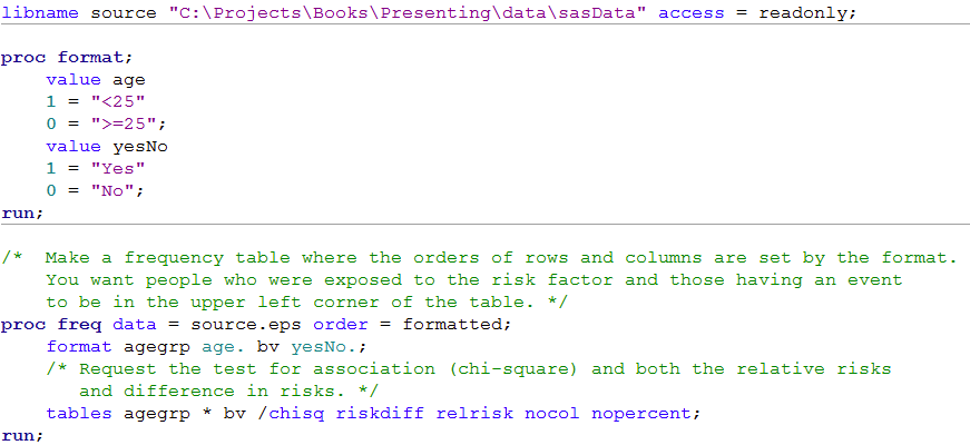
libname source "C:\Projects\Books\Presenting\data\sasData" access = readonly;

proc format;
    value age
    1 = "<25"
    0 = ">=25";
    value yesNo
    1 = "Yes"
    0 = "No";
run;

/*  Make a frequency table where the orders of rows and columns are set by the format.
    You want people who were exposed to the risk factor and those having an event
    to be in the upper left corner of the table. */
proc freq data = source.eps order = formatted;
    format agegrp age. bv yesNo.;
    /* Request the test for association (chi-square) and both the relative risks
       and difference in risks. */
    tables agegrp * bv /chisq riskdiff relrisk nocol nopercent;
run;
Figure 7.12 Output for odds ratio
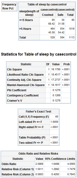
Figure 7.12 Code
 Click here to show code as text
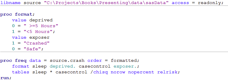
libname source "C:\Projects\Books\Presenting\data\sasData" access = readonly;

proc format;
    value deprived
    0 = " >=5 Hours"
    1 = "<5 Hours";
    value exposer
    1 = "Crashed"
    0 = "Safe";

proc freq data = source.crash order = formatted;
    format sleep deprived. casecontrol exposer.;
    tables sleep * casecontrol /chisq norow nopercent relrisk;
run;
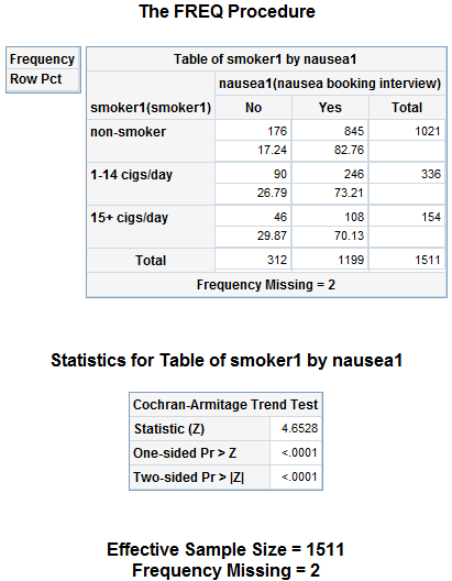
Table 7.1 Presenting ordered proportions
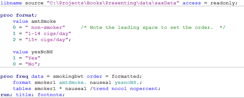
Box 7.12 Code
 Click here to show code as text
libname source "C:\Projects\Books\Presenting\data\sasData" access = readonly;

proc format;
    value amtSmoke
    0 = " non-smoker"     /* Note the leading space to set the order.  */
    1 = "1-14 cigs/day"
    2 = "15+ cigs/day";

    value yesNoNS
    1 = "Yes"
    0 = "No";

proc freq data = smokingbwt order = formatted;
    format smoker1 amtSmoke. nausea1 yesnoNS.;
    tables smoker1 * nausea1 /trend nocol nopercent;
run; title; footnote;