Chapter 7: Comparing two groups using SPSS
Figure 7.1
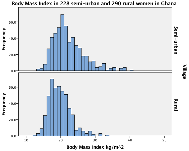
Figure 7.1 Instruction
Click here to show the instructions as text.
- Open the file.
- From the File menu choose Open > Data....
- Find the file ghana.sav and open it.
- Tell SPSS to display words instead of code numbers for the village location variable.
- Select the window showing the ghana dataset.
- Click on Variable View (at the bottom of the window).
- Click the Values box/cell next to the rural variable.
- Click on the ....
- In the Values box type 0.
- Type Semi-urban in Label box .
- Click Add.
- In the Values box type 1.
- In Label box type Rural.
- Click Add.
- Click OK.
- Tell SPSS to use good labels for the variable names.
- Select the window showing the ghana dataset.
- Click on Variable View (at the bottom of the window).
- Click the Label box/cell next to the rural variable.
- In the Label box type Village.
- Click the Label box/cell next to the BMI variable.
- Type Body Mass Index kg/m^2 in Label box.
- Tell SPSS to make a histogram.
- From the Graphics menu choose Chart Builder....
- If a window appears asking you to set measurement level, click OK.
- Click the Gallery button (in the lower part of the window).
- Click Histogram.
- Double click the left picture (the simple histogram).
- Drag BMI to the X-Axis? place holder in the graphic preview (the right windowpane).
- Click the Groups/Point ID button (in the lower part of the window).
- Check the Rows panel variable checkbox button.
- Drag rural to the Panel? place holder in the graphic preview.
- Click the Titles/Footnotes button.
- Check the Title 1 checkbox button.
- In the Element Properties window, in the Content: box, type Body Mass Index in 228 semi-urban and 290 rural women in Ghana.
- Click Apply.
- Click OK.
Figure 7.2

Figure 7.2 Instruction
SPSS does not have an automatic way to produce overlapping density plots.
Figure 7.3
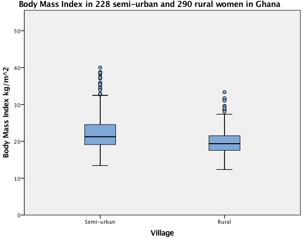
Figure 7.3 Instruction
Click here to show the instructions as text.
- Open the file.
- From the File menu choose Open > Data....
- Find the file ghana.sav and open it.
- Tell SPSS to display words instead of code numbers for the village location variable.
- Select the window showing the ghana dataset.
- Click on Variable View (at the bottom of the window).
- Click the Values box/cell next to the rural variable.
- Click on the ....
- In the Values box type 0.
- In Label box type Semi-urban .
- Click Add.
- In the Values box type 1 .
- In Label box type Rural.
- Click Add.
- Click OK.
- Tell SPSS to use good labels for the variable names.
- Select the window showing the ghana dataset.
- Click on Variable View (at the bottom of the window).
- Click the Label box/cell next to the rural variable.
- In the Label box type Village.
- Click the Label box/cell next to the BMI variable.
- In Label box type Body Mass Index kg/m^2.
- Tell SPSS to make boxplots.
- From the Graphics menu choose Chart Builder....
- If a window appears asking you to set measurement level, click OK.
- Click the Gallery button (in the lower part of the window).
- Click Boxplot.
- Double click the left picture (the simple boxplot).
- Drag rural to the X-Axis? place holder in the graphic preview (the right windowpane).
- Drag BMI to the y-Axis? place holder in the graphic preview.
- Click the Titles/Footnotes button (you may need to click the right facing triangle first).
- Check the Title 1 checkbox button.
- In the Element Properties window in the Content: box type Body Mass Index in 228 semi-urban and 290 rural women in Ghana.
- Click Apply.
- Click OK.
- Tell SPSS to remove the outlier labels.
- Double click the output boxplot table.
- Double click one of the labels.
- In the Properties window click the Data Value Labels button.
- In the Displayed: box click Case Number.
- Click the red x.
- Click Apply.
Figure 7.4

Figure 7.4 Instruction
SPSS does not have an automatic way to produce side by side violin plots.
Figure 7.5
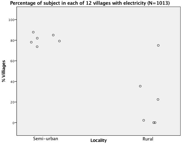
Figure 7.5 Instruction
Click here to show the instructions as text.SPSS does not have an automatic way to offset (jitter) overlapping data in only one direction. It is possible to make a new variable to plot and then manually edit the graphic.
- Open the file.
- From the File menu choose Open > Data....
- Find the file electricity.sav and open it.
- The locality (urbal vs. rural) is stored in a 0 vs. 1 indicator variable. We can add shift the values by up to + or -.15 to jitter the x axis.
- From the Transform menu choose Compute Variable....
- In the Target Variable: box type ruralJittered.
- Drag the rural variable to the Numeric Expression: box.
- In the Numeric Expression: box type +.
- In the Function group: box select Random Numbers.
- In the Functions and Special Variables: box double click Random Numbers.
- Replace the first ? following the ( with -.15 and the second ? with .15.
- Click OK.
- Tell SPSS to make a scatterplot.
- From the Graphics menu choose Chart Builder....
- If a window appears asking you to set measurement level, click OK.
- Click the Gallery button (in the lower part of the window).
- Click Scatter/Dot.
- Double click the left picture (the Simple Scatterplot).
- Drag ruralJittered to the X-Axis? place holder in the graphic preview (the right windowpane).
- Drag elec36 to the y-Axis? place holder in the graphic preview.
- Click the Titles/Footnotes button (you may need to click the right facing triangle first).
- Check the Title 1 checkbox button.
- In the Element Properties window in the Content: box type Percentage of subjects in each of 12 villages with electricity (N=1013).
- In the Element Properties window in the Edit Properties of: box select Y-Axis1(Point1).
- In the Axis Label: box type % Villiages.
- Click Apply.
- In the Element Properties window in the Content: box type Percentage of subjects in each of 12 villages with electricity (N=1013).
- Click Apply.
- Click OK.
- Click OK.
- Adjust the graphic.
- Double click the scatterplot.
- Double click the y-axis until the Properties window appears.
- In the Properties window in the Lower margin(%) box type 10.
- Click Apply.
- Double click the x-axis until the tick marks or labels are selected.
- In the Properties window click Labels & Ticks.
- Uncheck the Display labels box.
- Uncheck the Display ticks box.
- Click Apply.
- Where the Semi-urban label belongs, right click and choose Add Text Box.
- Type Semi-urban in the text box.
- Drag the Semi-urban text box to where it belongs.
- Where the Rural label belongs, right click and choose Add Text Box.
- Type Rural in the text box.
Figure 7.6

Figure 7.6 Instruction
Click here to show the instructions as text.
- Open the file.
- From the File menu choose Open > Data....
- Find the file pvd.sav and open it.
- Tell SPSS to make a histogram.
- From the Graphics menu choose Chart Builder....
- If a window appears asking you to set measurement level, click OK.
- Click the Gallery button (in the lower part of the window).
- Click Histogram.
- Double click the left picture (the simple histogram).
- Drag sbp to the X-Axis? place holder in the graphic preview (the right windowpane).
- In the Edit Properties of: window click Bar1 if it is not highlighed.
- Check on the Display normal curve checkbox.
- Click Apply.
- In the Edit Properties of: window click X-Axis1(Bar1).
- In the Axis label: box type Histogram of systolic blood presure with a normal distribution curve.
- Click Apply.
- Click OK.
Figure 7.7

Figure 7.7 Instruction
Click here to show the instructions as text.
- Open the file.
- From the File menu choose Open > Data....
- Find the file pvd.sav and open it.
- Tell SPSS to display words instead of secret code numbers for the outcome variable.
- Select the window showing the pvd dataset.
- Click on Variable View (at the bottom of the window).
- Click the Values box/cell for the outcome variable.
- Click on the ....
- In the Values: box type 0.
- In the Label: box type Dead.
- Click Add.
- In the Values: box type 1.
- In the Label: box type Alive.
- Click Add.
- Click OK.
- Tell SPSS to do a two sample t-test.
- From the Analyze menu choose Compare Means > Independent-Samples T Test....
- Drag sbp to the Test Variable(s): box.
- Drag outcome to the Grouping Variable: box.
- Click Define Groups....
- In the Group 1: box type 0.
- In the Group 2: box type 1.
- Click Continue.
- Click OK.
Figure 7.8
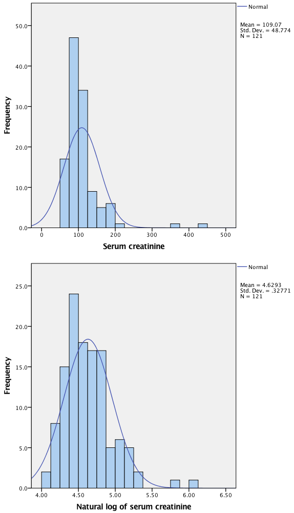
Figure 7.8 Instruction
Click here to show the instructions as text.
- Open the file.
- From the File menu choose Open > Data....
- Find the file pvd.sav and open it.
- Open the file.
- From the File menu choose Open > Data....
- Find the file pvd.sav and open it.
- Tell SPSS to compute a natural log transformed version of serum creatinine.
- From the Transform menu choose Compute Variable....
- In the Target Variable: box type lnCR.
- In the Function group: box select Arithmetic.
- In the Functions and Special Variables: box double click Ln.
- Double click on cr.
- Click OK.
- Tell SPSS to make a histogram.
- From the Graphics menu choose Chart Builder....
- If a window appears asking you to set measurement level, click OK.
- Click the Gallery button (in the lower part of the window).
- Click Histogram.
- Double click the left picture (the simple histogram).
- Drag cr to the X-Axis? place holder in the graphic preview (the right windowpane).
- In the Edit Properties of: window click Bar1 if it is not highlighed.
- Check on the Display normal curve checkbox.
- Click Apply.
- In the Edit Properties of: window click X-Axis1(Bar1).
- In the Axis label: box type Serum creatinine.
- Click Apply.
- Click OK.
- Tell SPSS to make a second histogram.
- From the Graphics menu choose Chart Builder....
- If a window appears asking you to set measurement level, click OK.
- Click the Gallery button (in the lower part of the window).
- Click Histogram.
- Double click the left picture (the simple histogram).
- Drag lnCR to the X-Axis? place holder in the graphic preview (the right windowpane).
- In the Edit Properties of: window click Bar1 if it is not highlighed.
- Check on the Display normal curve checkbox.
- Click Apply.
- In the Edit Properties of: window click X-Axis1(Bar1).
- In the Axis label: box type Natural log of serum creatinine.
- Click Apply.
- Click OK.
The log transformed variable is already in the dataset. Do the following to see how it was created.
Figure 7.9 and Box 7.4

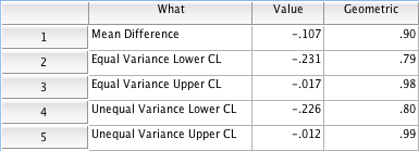
Figure 7.9 Instruction
Click here to show the instructions as text.SPSS does not have the ability to automatically calculate the geometric mean. The steps below show a way to get the mean and 95% confidence limits.
- Open the file.
- From the File menu choose Open > Data....
- Find the file rhinitis.sav and open it.
- Tell SPSS to display words instead of secret code numbers for the outcome variable.
- Select the window showing the pvd dataset.
- Click on Variable View (at the bottom of the window).
- Click the Values box/cell for the outcome variable.
- Click on the ....
- In the Values: box type 0.
- In the Label: box type Dead.
- Click Add.
- In the Values: box type 1.
- In the Label: box type Alive.
- Click Add.
- Click OK.
- Tell SPSS to do a two sample t-test.
- From the Analyze menu choose Compare Means > Independent-Samples T Test....
- Drag lcr to the Test Variable(s): box.
- Drag outcome to the Grouping Variable: box.
- Click Define Groups....
- In the Group 1: box type 0.
- In the Group 2: box type 1.
- Click Continue.
- Click OK.
- Make a new dataset that will hold the transformed versions of the mean and CLs.
- From the File menu choose New> Data.
- Click on Variable View (at the bottom of the window).
- Click the Name box/cell for the 1st row.
- Type What .
- Click the Type box/cell next to where you wrote What.
- Click on the ....
- Click on the String radio button.
- In the Characters: box type 25.
- Click OK.
- Click the Name box/cell for the 2nd row.
- Type Value .
- Click the Decimals box/cell for the 2nd row.
- Type 3.
- Click on Data View (at the bottom of the window).
- In the first row, in the What cell, type Mean Difference.
- In the first row, in the Value cell, type -.107.
- In the second row, in the What cell, type Equal Variance Lower CL.
- In the second row, in the Value cell, type -.231.
- In the third row, in the What cell, type Equal Variance Upper CL.
- In the third row, in the Value cell, type -.017.
- In the fourth row, in the What cell, type Unequal Variance Lower CL.
- In the fourth row, in the Value cell, type -.226.
- In the fifth row, in the What cell, type Unequal Variance Upper CL.
- In the fifth row, in the Value cell, type -.012.
- Tell SPSS to compute the antilog of the mean and CLs.
- From the Transform menu choose Compute Variable....
- In the Target Variable: box type Geometric.
- In the Function group: box select Arithmetic.
- In the Functions and Special Variables: box double click Exp.
- Double click on Value.
- Click OK.
Figure 7.10

... or with descriptive statistics
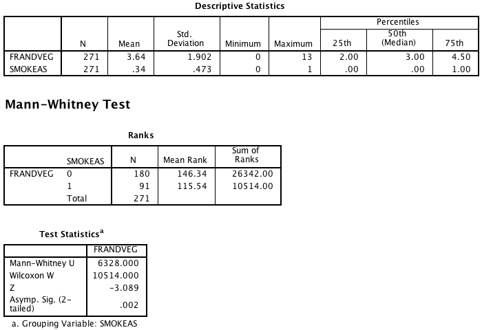
Figure 7.10 Instruction
Click here to show the instructions as text.There are two ways to do the analysis. The legacy method gives some additional descriptive statistics.
- Open the file.
- From the File menu choose Open> Data....
- Find the file eat.sav and open it.
- Tell SPSS to compare the distributions (without extra descriptive statistics).
- From the Analyze menu choose Nonparametric Tests > Independent Samples....
- Click the Objective button (at the top of the window).
- Confirm that Automatically compare distributions across groups is selected.
- Click the Fields button (at the top of the window).
- Drag frandveg into the Test Fields: box.
- Drag smokeas into the Groups: box.
- Click the Run button.
- Tell SPSS to compare the distributions (along extra descriptive statistics).
- From the Analyze menu choose Nonparametric Tests> Legacy Dialogs> 2 Independent Samples.
- Drag frandveg into the Test Variable List: box.
- Drag smokeas into the Grouping Variable: box.
- Click the Define Groups... button.
- In the Group 1: box type 0.
- In the Group 2: box type 1.
- Click the Continue button.
- Click the Options... button.
- In the Statistics section check the Descriptive and Quartiles checkboxes.
- Click the Continue button.
- Click the OK button.
Figure 7.11
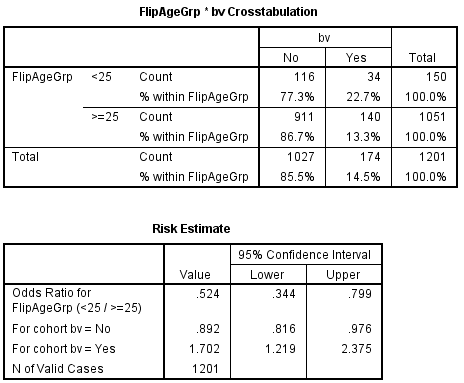
Figure 7.11 Instruction
Click here to show the instructions as text.
- Open the file.
- From the File menu choose Open> Data....
- Find the file eps.sav and open it.
- Specify that you want to convert outcome variable so the presence of the predictor is first in alphabetic order. Here has BV comes before no BV..
- From the Transform menu choose Recode into different variables... .
- Drag bv to the String Variable -> Output Varible: box.
- Click Old and New Values... .
- Type 0 in the Old Value Value: box.
- Check on the Output variables are string checkbox.
- Type no BV in the New Value Value: box.
- Click Add.
- Type 1 in the Old Value Value: box.
- Type has BV in the New Value Value: box.
- Click Add.
- Click Continue.
- Type hasBV in the Output Variable Name: box.
- Type BV Status in the Output Label Name: box.
- Click Change.
- Click OK.
- Specify that you want to convert the predictor variable so the presence of the risk factor is first in alphabetic order. Here Old comes before Young..
- Drag ageGrp to the String Variable -> Output Varible: box.
- Click Old and New Values... .
- Type 0 in the Old Value Value: box.
- Check on the Output variables are string checkbox.
- Type Young in the New Value Value: box.
- Click Add.
- Type 1 in the Old Value Value: box.
- Type Old in the New Value Value: box.
- Click Add.
- Click Continue.
- Type ageGrpString in the Output Variable Name: box.
- Type Age group in the Output Label Name: box.
- Click Change.
- Click OK.
- Tell SPSS to make a dataset with no missing data.
- From the Data menu choose Select Cases... .
- Click the If condition is satisfied radio button.
- Click the If... button.
- In the box at the top of the window type hasBV ~= "".
- Click Continue.
- Click OK.
- Tell SPSS to do a cross tabulation.
- From the Analyze menu choose Descriptive Statistics > Crosstabs....
- Drag Age to the Rows(s) box.
- Drag BV to the Column(s) box.
- Click Statistics....
- Check/tick the Risk checkbox/tickbox.
- Click Continue.
- Click Cells....
- In the Percentages section check/tick the Rows checkbox/tickbox.
- Click Continue.
- Click OK.
Figure 7.12
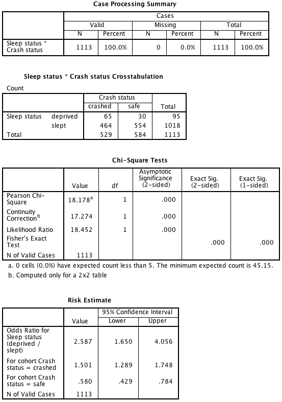
Figure 7.12 Instruction
Click here to show the instructions as text.
- Open the file.
- From the File menu choose Open> Data....
- Find the file crash.sav and open it.
- Specify that you want to convert the outcome variable so the presence of the event is first in alphabetic order. Here crashed comes before safe..
- Drag ageGrp to the String Variable -> Output Varible: box.
- Click Old and New Values... .
- Type 0 in the Old Value Value: box.
- Check on the Output variables are string checkbox.
- Type safe in the New Value Value: box.
- Click Add.
- Type 1 in the Old Value Value: box.
- Type crashed in the New Value Value: box.
- Click Add.
- Click Continue.
- Type crashed in the Output Variable Name: box.
- Type Crash status in the Output Label Name: box.
- Click Change.
- Click OK.
- Specify that you want to convert the predictor variable so the presence of the predictor is first in alphabetic order. Here deprived comes before slept.
- From the Transform menu choose Recode into different variables....
- Drag sleep to the String Variable -> Output Varible: box.
- Click Old and New Values... .
- Type 0 in the Old Value Value: box.
- Check on the Output variables are string checkbox.
- Type slept in the New Value Value: box.
- Click Add.
- Type 1 in the Old Value Value: box.
- Type deprived in the New Value Value: box.
- Click Add.
- Click Continue.
- Type deprived in the Output Variable Name: box.
- Type Sleep Status in the Output Label Name: box.
- Click Change.
- Click OK.
- Tell SPSS to do a cross tabulation.
- From the Analyze menu choose Descriptive Statistics > Crosstabs ....
- Drag deprived to the Rows(s) box.
- Drag crashed to the Column(s) box.
- Click Statistics....
- Check on the Chi-square checkbox.
- Check on the Risk checkbox.
- Click Continue.
- Click Cells....
- In the Percentages section check on the Rows checkbox.
- Click Continue.
- Click OK.
Box 7.12

Box 7.12 Instruction
SPSS does not automatically produce a Cochran-Armitage test for trend