Chapter 8: Analysing matched or paired data using R
Figure 8.1 Output for a paired t-test
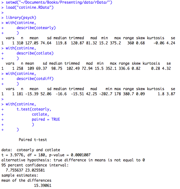
Figure 8.1 Code
Click here to show code with comments# Tell R where you will be working. R will look here for your data: setwd("~/Documents/Books/Presenting/data/rData/") # See chapter 2 for more details on the setwd() funciton. # Use the load() function to load the dataset cotinine.RData out of the current # folder/directory into R's interactive working memory/environment. See chapter # 2 for more details. load("cotinine.RData") # See chapter 2 for a discussion of the library function. library(psych) # load psych to get its describe function with(cotinine, describe(cotearly) ) with(cotinine, describe(cotlate) ) with(cotinine, describe(cotdiff) # Note the negative values in the output. The cotdiff # late - early is a negative value. The data could # be presented as a reduction (with a negative value) # or as a difference (without the negative). ) # See the code for chapter 5 for a discussion of the with() function. This code # could also be written as: # # t.test(hasDiff$cotearly, hasDiff$cotlate, paired = TRUE) # # The t.test() function can be used to test whether the difference in paired # values is zero. with(cotinine, # the data frame t.test(cotearly, # One of the measurements cotlate, # The other measurement paired = TRUE # Indicate that this study uses repeated measures on # the same subjects. ) )
Figure 8.2 Histogram of skewed paired data (a) before and (b) after log transformation with normal distribution curve
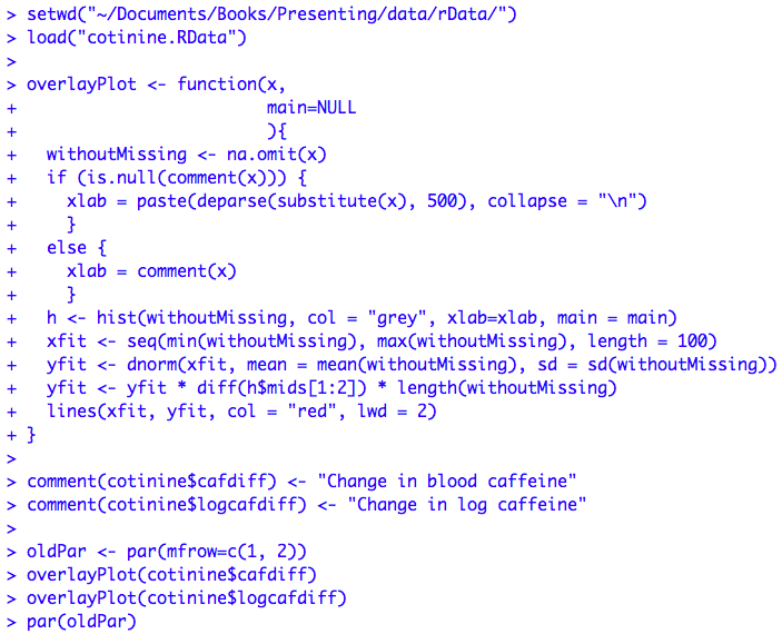
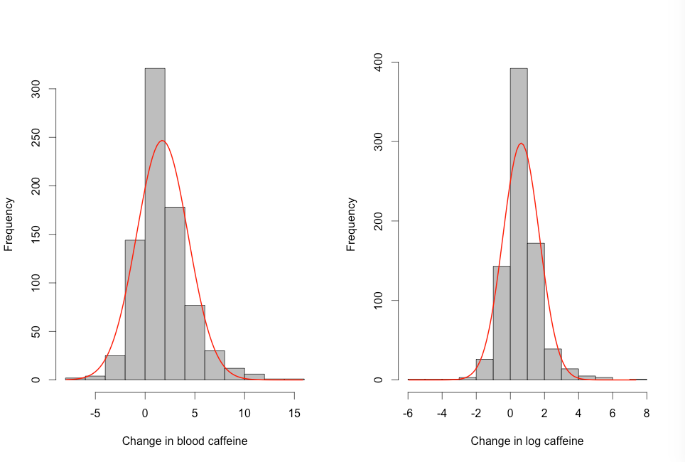
Figure 8.2 Code
Click here to show code with comments# Figure 8.4 setwd("~/Documents/Books/Presenting/data/rData/") load("cotinine.RData") # The function() function is used to create a user-defined function called # overlayPlot which will allow two arguments. The x parameter is the variable # to be plotted and main is the parameter used to indicate the title, which # defaults to being blank. The drawing part of this code is documented in # chapter 7. This uses the na.omit() function to remove missing values. See # chapter 2 for more details on comment(). It is good form to use the comment() # function to document your variables. Here, the code checks to see if the # variable has a comment and if it exists, it is used to label the x-axis. If # there is no label, it uses the variable name. overlayPlot <- function(x, # This is the variable to be plotted. main=NULL # Use the main argument to add a title. ){ withoutMissing <- na.omit(x) # The is.null() function checks to see if there is a comment associated # with the variable passed to (used by) the function and it returns true or # false. The if() function does the action inside of { } if the is.null() # returns TRUE. Otherwise, the actions defined in { } after the else are done. if (is.null(comment(x))) { # This combination of deparse() and substitute() functions can be used to # get the name of the variable passed to the function. The paste function is # used to remove any "new line" characters that could be passed with the # variable name. xlab = paste(deparse(substitute(x), 500), collapse = "\n") } else { xlab = comment(x) } h <- hist(withoutMissing, col = "grey", xlab=xlab, main = main) xfit <- seq(min(withoutMissing), max(withoutMissing), length = 100) yfit <- dnorm(xfit, mean = mean(withoutMissing), sd = sd(withoutMissing)) yfit <- yfit * diff(h$mids[1:2]) * length(withoutMissing) lines(xfit, yfit, col = "red", lwd = 2) } comment(cotinine$cafdiff) <- "Change in blood caffeine" comment(cotinine$logcafdiff) <- "Change in log caffeine" # The par() function can be used to set many options for many graphics. To learn # more about par() look here: # http://www.statmethods.net/advgraphs/layout.html # http://www.statmethods.net/advgraphs/parameters.html # # From now on, every two plots go into two columns in one image. With this # syntax, the object called oldPar will automatically store the old values of # the mfrow option. oldPar <- par(mfrow=c(1, 2)) overlayPlot(cotinine$cafdiff) overlayPlot(cotinine$logcafdiff) par(oldPar)
Figure 8.3 Paired t-test with back-transformation
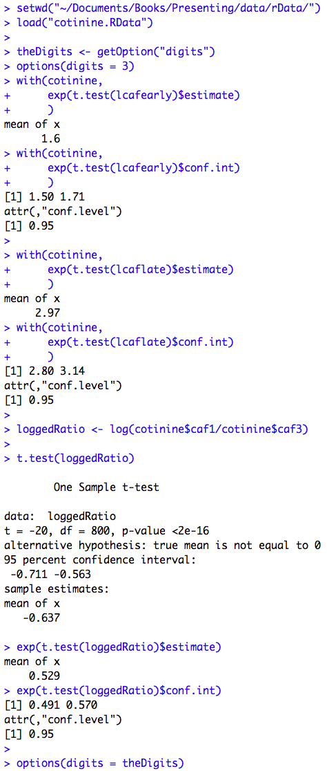
Figure 8.3 Code
Click here to show code with commentssetwd("~/Documents/Books/Presenting/data/rData/") load("cotinine.RData") # The getOption() function can be used to see R's global options, such as the # number of decimal places shown. Here, getOption() is used to get and save # the current number of digits used in rounding results. This is done so the # display option can be reset later. theDigits <- getOption("digits") # The options function can be used to set R's global options. options(digits = 3) # Set output to round to 3 digits. # Do a t-test to get the confidence limits on the mean. It also gives the mean. with(cotinine, # The exp() function calculates the exponential function. exp(t.test(lcafearly)$estimate) # Exponentiate the observed mean. ) with(cotinine, exp(t.test(lcafearly)$conf.int) # Exponentiate the confidence limits. ) with(cotinine, exp(t.test(lcaflate)$estimate) ) with(cotinine, exp(t.test(lcaflate)$conf.int) ) # The log() function computes logarithms. Here it is used to make a new # variable/vector called loggedRatio that has the logged ratio of the early and # late caffeine levels. loggedRatio <- log(cotinine$caf1/cotinine$caf3) t.test(loggedRatio) # Look at the t-test. exp(t.test(loggedRatio)$estimate) # Exponentiate the observed mean. exp(t.test(loggedRatio)$conf.int) # Exponentiate the confidence limits. options(digits = theDigits) # Reset the rounding to the original value.
Figure 8.4 Output for a Wilcoxon matched pairs test

Figure 8.4
Click here to show code with comments
R code goes here
Box 8.7 Presenting the findings of the Wilcoxon test for matched pairs
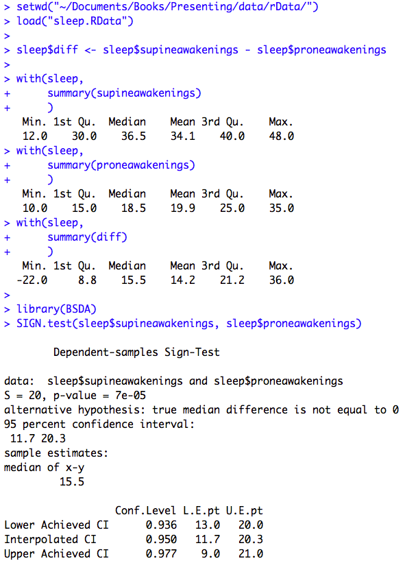
Box 8.7
Click here to show code with commentssetwd("~/Documents/Books/Presenting/data/rData/") load("sleep.RData") # Calculate the difference in the number of awakenings by sleeping position. sleep$diff <- sleep$supineawakenings - sleep$proneawakenings with(sleep, summary(supineawakenings) # Get median and quartiles. ) with(sleep, summary(proneawakenings) ) with(sleep, summary(diff) ) # Load the BSDA package to get the SIGN.test() function. library(BSDA) SIGN.test(sleep$supineawakenings, sleep$proneawakenings)
Figure 8.5 Output for a matched case-control analysis
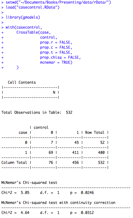
Figure 8.5 Code
Click here to show code with commentsBox 8.10 Asthma case-control study
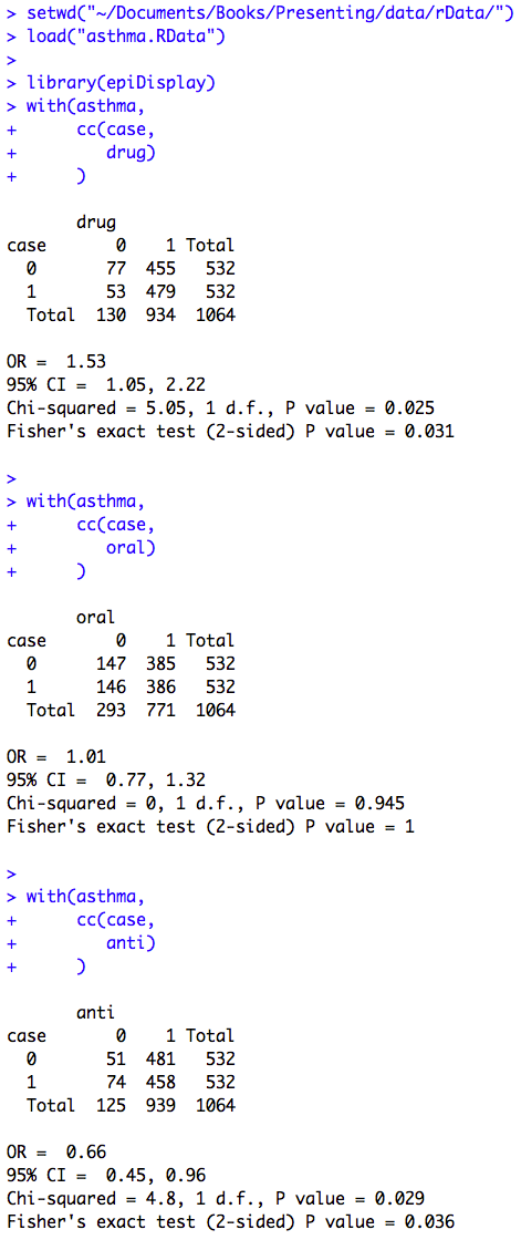
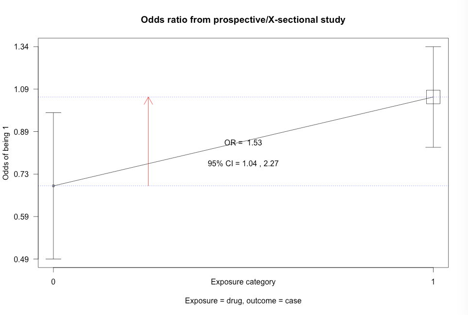
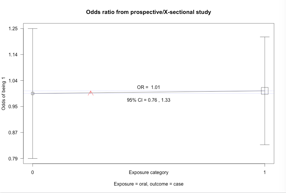
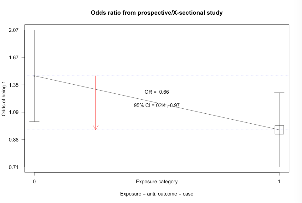
Box 8.10 Code
Click here to show code with commentssetwd("~/Documents/Books/Presenting/data/rData/") load("asthma.RData") library(epiDisplay) # Use the epiDisplay package to get the cc() function. # Use the cc() function to calculate an odds ratio with exact CL, chi-square and # Fisher's exact test. with(asthma, # case-control studies cc(case, # outcome 1 = yes drug) # predictor 1 = yes ) with(asthma, cc(case, oral) ) with(asthma, cc(case, anti) )
Figure 8.6 Output for McNemar’s test with ratio of paired proportions
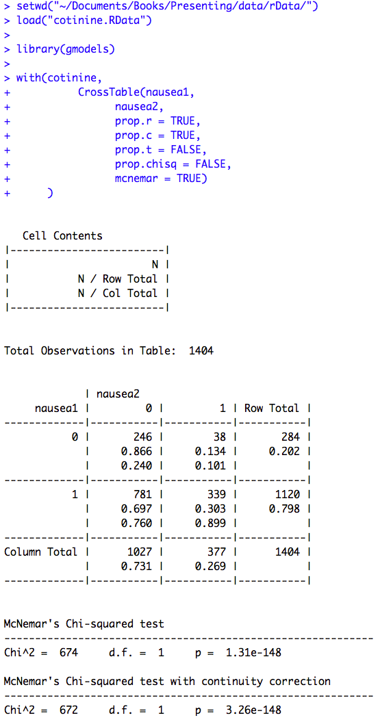
Figure 8.6 Code
Click here to show code with commentssetwd("~/Documents/Books/Presenting/data/rData/") load("cotinine.RData") # Load the gmodels package to get the fancy CrossTable() function. library(gmodels) with(cotinine, # The CrossTable() function generates frequency tables and it can do many common # cross tabulation statistics. CrossTable(nausea1, nausea2, prop.r = TRUE, prop.c = TRUE, prop.t = FALSE, prop.chisq = FALSE, mcnemar = TRUE) )