Chapter 8: Analysing matched or paired data using SAS
Figure 8.1 Output for a paired t-test
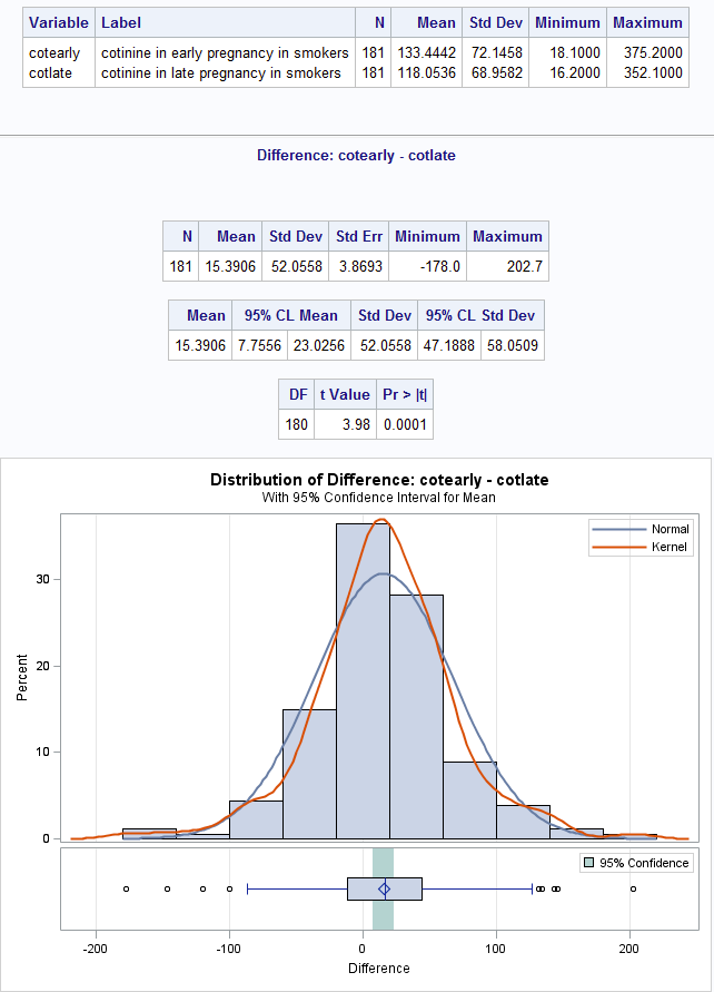
Figure 8.1 Code
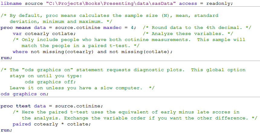 Click here to show code as text
libname source "C:\Projects\Books\Presenting\data\sasData" access = readonly;

/* By default, proc means calculates the sample size (N), mean, standard
   deviation, minimum and maximum. */
proc means data = source.cotinine maxdec = 4;  /* Round data to the 4th decimal. */
    var cotearly cotlate;                      /* Analyze these variables. */
    /* Only include people who have both cotinine measurements.  This sample will
       match the people in a paired t-test. */
    where not missing(cotearly) and not missing(cotlate);
run;

/* The "ods graphics on" statement requests diagnostic plots.  This global option
   stays on until you type:
        ods graphics off;
   Leave it on unless you have a slow computer.  */
ods graphics on;

proc ttest data = source.cotinine;
    /* Here the paired t-test uses the equivalent of early minus late scores in
       the analysis. Exchange the variable order if you want the other difference. */
    paired cotearly * cotlate;
run;
Figure 8.2 Histogram of skewed paired data (a) before and (b) after log transformation with normal distribution curve
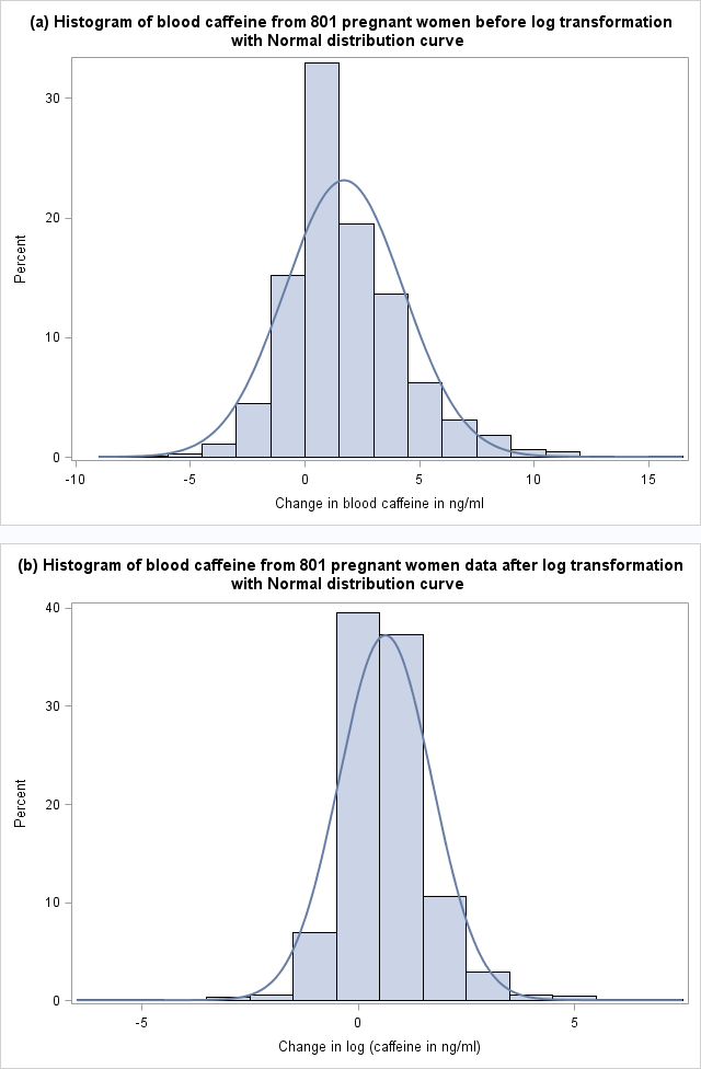
Figure 8.2 Code
 Click here to show code as text
libname source "C:\Projects\Books\Presenting\data\sasData" access = readonly;

proc sgplot data = source.cotinine noautolegend;  /* noautolegend turns off the key/legend. */
    title "(a) Histogram of blood caffeine from 801 pregnant women before log transformation with Normal distribution curve";
    label cafdiff = "Change in blood caffeine in ng/ml";
    histogram cafdiff;
    density cafdiff;  /* Draw a normal/Gaussian density curve. */
run; title;

proc sgplot data = source.cotinine noautolegend;
    title "(b) Histogram of blood caffeine from 801 pregnant women data after log transformation with Normal distribution curve";
    label logcafdiff = "Change in log (caffeine in ng/ml)";
    histogram logcafdiff;
    density logcafdiff;
run;
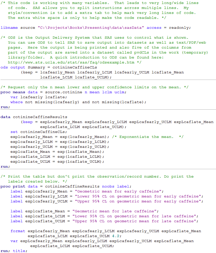
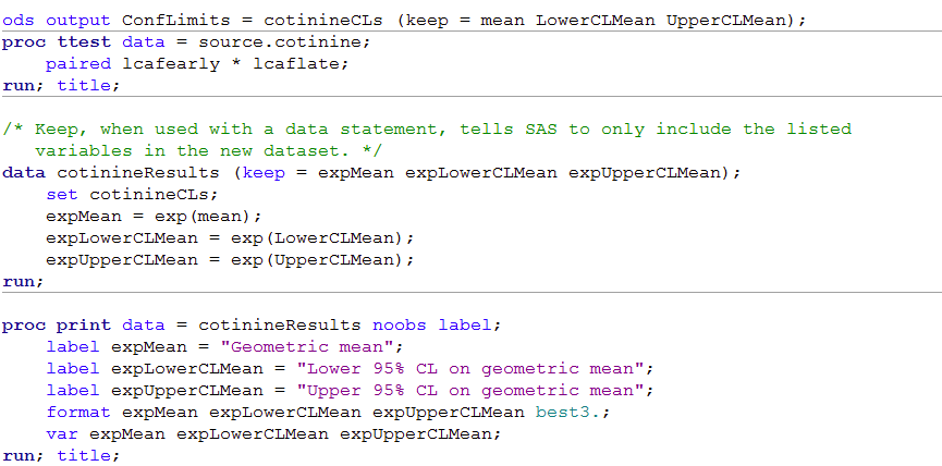
Figure 8.3 Output for back transforming t-test data
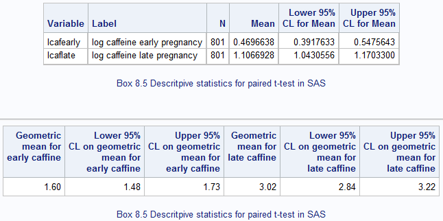
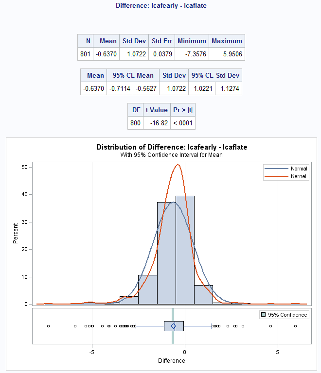
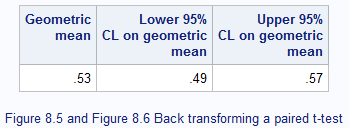
Figure 8.3 Code
 Click here to show code as text
/* This code is working with many variables.  That leads to very long/wide lines
   of code.  SAS allows you to split instructions across multiple lines.  My
   style/convention is to add a extra tab to help mark very long lines of code.
   The extra white space is only to help make the code readable. */

libname source "C:\Projects\Books\Presenting\data\sasData" access = readonly;

/* ODS is the Output Delivery System that SAS uses to control what is shown.
   You can use ODS to tell SAS to save output into datasets as well as text/PDF/web
   pages.  Here the output is being printed and also five of the columns from
   part of the output are saved into a dataset called pvdCLs in the work (temporary)
   library/folder.  A quick introduction to ODS can be found here:
   http://www.ats.ucla.edu/stat/sas/faq/odsexample.htm */
ods output Summary = cotinineCaffineCLs
        (keep = lcafearly_Mean lcafearly_LCLM lcafearly_UCLM lcaflate_Mean
                lcaflate_LCLM lcaflate_UCLM);

/* Request only the n mean lower and upper confidence limits on the mean. */
proc means data = source.cotinine n mean lclm uclm;
    var lcafearly lcaflate;
    where not missing(lcafearly) and not missing(lcaflate);
run;

data cotinineCaffineResults
        (keep = expLcafearly_Mean expLcafearly_LCLM expLcafearly_UCLM expLcaflate_Mean
                expLcaflate_LCLM expLcaflate_UCLM);
    set cotinineCaffineCLs;
    explcafearly_Mean = exp(lcafearly_Mean); /* Exponentiate the mean.  */
    explcafearly_LCLM = exp(lcafearly_LCLM);
    explcafearly_UCLM = exp(lcafearly_UCLM);
    explcaflate_Mean = exp(lcaflate_Mean);
    explcaflate_LCLM = exp(lcaflate_LCLM);
    explcaflate_UCLM = exp(lcaflate_UCLM);
run;

/* Print the table but don't print the observation/record number. Do print the
   labels created below. */
proc print data = cotinineCaffineResults noobs label;
    label explcafearly_Mean = "Geometric mean for early caffeine";
    label explcafearly_LCLM = "Lower 95% CL on geometric mean for early caffeine";
    label explcafearly_UCLM = "Upper 95% CL on geometric mean for early caffeine";

    label explcaflate_Mean = "Geometric mean for late caffeine";
    label explcaflate_LCLM = "Lower 95% CL on geometric mean for late caffeine";
    label explcaflate_UCLM = "Upper 95% CL on geometric mean for late caffeine";

    format expLcafearly_Mean expLcafearly_LCLM expLcafearly_UCLM expLcaflate_Mean
           expLcaflate_LCLM expLcaflate_UCLM 4.2;
    var expLcafearly_Mean expLcafearly_LCLM expLcafearly_UCLM expLcaflate_Mean
            expLcaflate_LCLM expLcaflate_UCLM;
run; title;

ods output ConfLimits = cotinineCLs (keep = mean LowerCLMean UpperCLMean);
proc ttest data = source.cotinine;
    paired lcafearly * lcaflate;
run; title;

/* Keep, when used with a data statement, tells SAS to only include the listed
   variables in the new dataset. */
data cotinineResults (keep = expMean expLowerCLMean expUpperCLMean);
    set cotinineCLs;
    expMean = exp(mean);
    expLowerCLMean = exp(LowerCLMean);
    expUpperCLMean = exp(UpperCLMean);
run;

proc print data = cotinineResults noobs label;
    label expMean = "Geometric mean";
    label expLowerCLMean = "Lower 95% CL on geometric mean";
    label expUpperCLMean = "Upper 95% CL on geometric mean";
    format expMean expLowerCLMean expUpperCLMean best3.;
    var expMean expLowerCLMean expUpperCLMean;
run; title;
Figure 8.4 Output for a Wilcoxon matched pairs test

Figure 8.4 Code
 Click here to show code as text
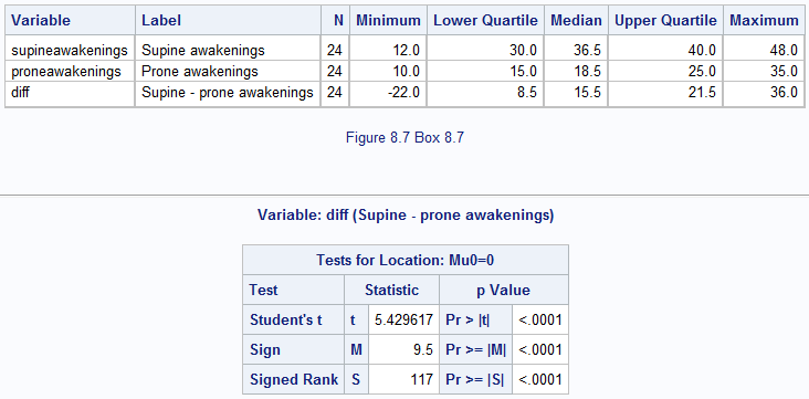
Box 8.7 Presenting the findings of the Wilcoxon test for matched pairs
Box 8.7 Code
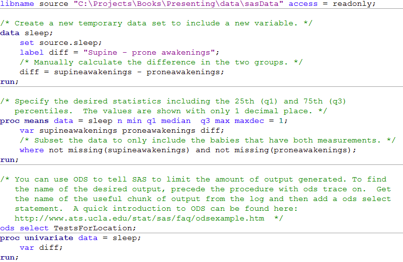 Click here to show code as text
libname source "C:\Projects\Books\Presenting\data\sasData" access = readonly;

/* Create a new temporary data set to include a new variable. */
data sleep;
    set source.sleep;
    label diff = "Supine - prone awakenings";
    /* Manually calculate the difference in the two groups. */
    diff = supineawakenings - proneawakenings;
run;

/* Specify the desired statistics including the 25th (q1) and 75th (q3)
   percentiles.  The values are shown with only 1 decimal place. */
proc means data = sleep n min q1 median  q3 max maxdec = 1;
    var supineawakenings proneawakenings diff;
    /* Subset the data to only include the babies that have both measurements. */
    where not missing(supineawakenings) and not missing(proneawakenings);
run;

/* You can use ODS to tell SAS to limit the amount of output generated. To find
   the name of the desired output, precede the procedure with ods trace on.  Get
   the name of the useful chunk of output from the log and then add a ods select
   statement.  A quick introduction to ODS can be found here:
   http://www.ats.ucla.edu/stat/sas/faq/odsexample.htm  */
ods select TestsForLocation;
proc univariate data = sleep;
    var diff;
run;
Figure 8.5 Output for a matched case-control analysis
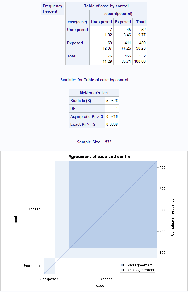
Figure 8.5 Code
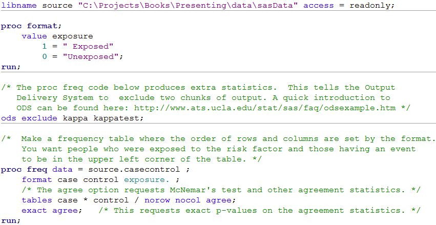 Click here to show code as text
libname source "C:\Projects\Books\Presenting\data\sasData" access = readonly;

proc format;
    value exposure
        1 = " Exposed"
        0 = "Unexposed";
run;

/* The proc freq code below produces extra statistics.  This tells the Output
   Delivery System to  exclude two chunks of output. A quick introduction to
   ODS can be found here: http://www.ats.ucla.edu/stat/sas/faq/odsexample.htm */
ods exclude kappa kappatest;

/*  Make a frequency table where the order of rows and columns are set by the format.
    You want people who were exposed to the risk factor and those having an event
    to be in the upper left corner of the table. */
proc freq data = source.casecontrol ;
    format case control exposure. ;
    /* The agree option requests McNemar's test and other agreement statistics. */
    tables case * control / norow nocol agree;
    exact agree;   /* This requests exact p-values on the agreement statistics. */
run;
Box 8.10 Presenting the results of matched case-control analysis
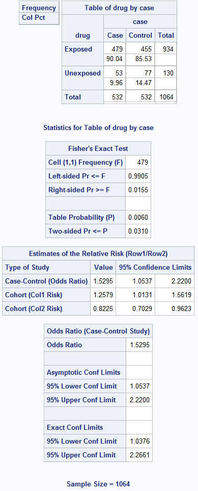
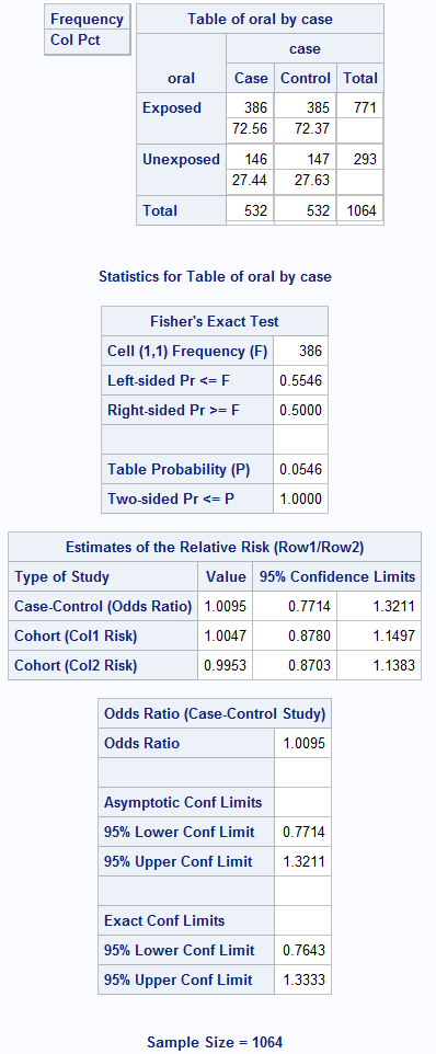
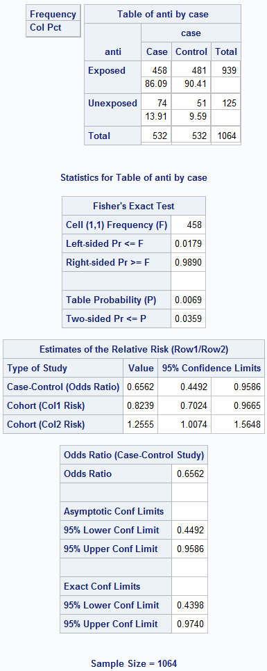
Box 8.10 Code
 Click here to show code as text
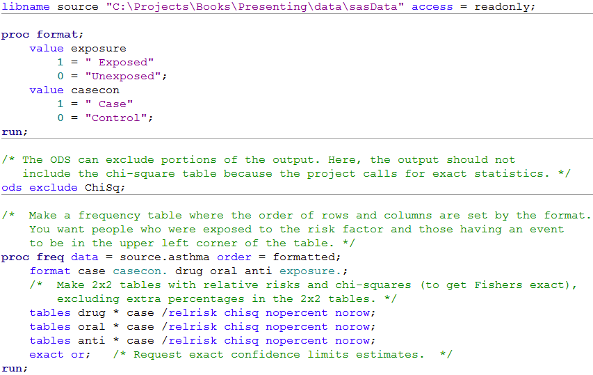
libname source "C:\Projects\Books\Presenting\data\sasData" access = readonly;

proc format;
    value exposure
        1 = " Exposed"
        0 = "Unexposed";
    value casecon
        1 = " Case"
        0 = "Control";
run;

/* The ODS can exclude portions of the output. Here, the output should not
   include the chi-square table because the project calls for exact statistics. */
ods exclude ChiSq;

/*  Make a frequency table where the order of rows and columns are set by the format.
    You want people who were exposed to the risk factor and those having an event
    to be in the upper left corner of the table. */
proc freq data = source.asthma order = formatted;
    format case casecon. drug oral anti exposure.;
    /*  Make 2x2 tables with relative risks and chi-squares (to get Fishers exact),
        excluding extra percentages in the 2x2 tables. */
    tables drug * case /relrisk chisq nopercent norow;
    tables oral * case /relrisk chisq nopercent norow;
    tables anti * case /relrisk chisq nopercent norow;
    exact or;   /* Request exact confidence limits estimates.  */
run;
Figure 8.6 Output for McNemar’s test with ratio of paired proportions
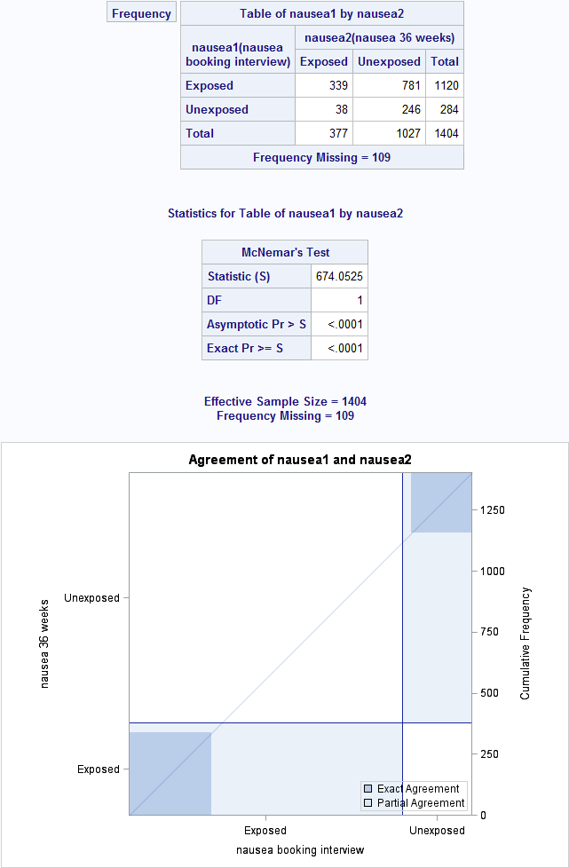
Figure 8.6 Code
 Click here to show code as text
libname source "C:\Projects\Books\Presenting\data\sasData" access = readonly;

proc format;
    value exposure
        1 = " Exposed"  /* Note the leading space.  This sets the row/column
                           order below */
        0 = "Unexposed";

proc freq data = source.cotinine order = formatted;
    format nausea1 nausea2 exposure. ;
    tables nausea1 * nausea2 / agree ;
    exact agree;
run;