Chapter 8: Analyzing matched or paired data using SPSS
Figure 8.1 Output for a paired t-test
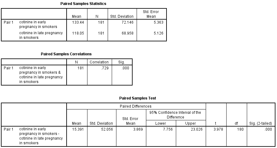
Figure 8.1 Instruction
Click here to show the instructions as text.
- Open the file.
- From the File menu choose Open> Data....
- Find the file cotinine.sav and open it.
- Tell SPSS to compare the means of two related samples with a paired t-test.
- From the Analyze menu choose Compare Means > Paired-Samples T Test....
- Drag cotearly to the Paired Variables: box.
- Drag cotlate to the Paired Variables: box.
- Click OK.
Figure 8.2 Histogram of skewed paired data (a) before and (b) after log transformation with normal distribution curve
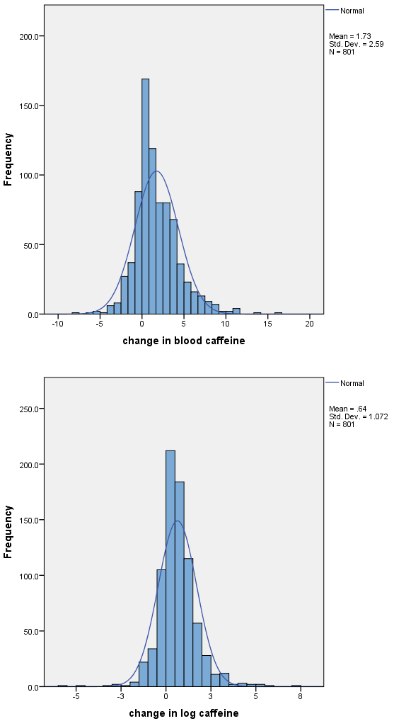
Figure 8.2 Instruction
Click here to show the instructions as text.
- Open the file.
- From the File menu choose Open> Data....
- Find the file cotinine.sav and open it.
- Tell SPSS to make a histogram.
- From the Graphics menu choose Chart Builder....
- If a window appears asking you to set measurement level, click OK.
- Click the Gallery button (in the lower part of the window).
- Click Histogram.
- Double click the left picture (the simple histogram).
- Drag cafdiff to the X-Axis? place holder in the graphic preview (the right windowpane).
- In the Edit Properties of: window click Bar1 if it is not highlighed.
- Check on the Display normal curve checkbox.
- Click Apply.
- In the Edit Properties of: window click X-Axis1(Bar1).
- In the Axis label: box type Change in blood caffeine in ng/ml.
- Click Apply.
- In the Chart Builder window push the Titles/Footnotes button.
- Check on the Title 1 checkbox.
- In the Element Properties window, in the Content: box, type (a) Histogram of blood caffeine from 801 pregnant women before log transformation with normal distribution curve.
- Click OK.
- Tell SPSS to make a second histogram.
- From the Graphics menu choose Chart Builder....
- If a window appears asking you to set measurement level, click OK.
- Click the Gallery button (in the lower part of the window).
- Click Histogram.
- Double click the left picture (the simple histogram).
- Drag logcafdiff to the X-Axis? place holder in the graphic preview (the right windowpane).
- In the Edit Properties of: window click Bar1 if it is not highlighed.
- Check on the Display normal curve checkbox.
- Click Apply.
- In the Edit Properties of: window click X-Axis1(Bar1).
- In the Axis label: box type Change in log (caffeine in ng/ml).
- Click Apply.
- In the Chart Builder window push the Titles/Footnotes button.
- Check on the Title 1 checkbox.
- In the Element Properties window, in the Content: box, type (b) Histogram of blood caffeine from 801 pregnant women data after log transformation with normal distribution curve.
- Click OK.
Figure 8.3 Paired t-test with back-transformation
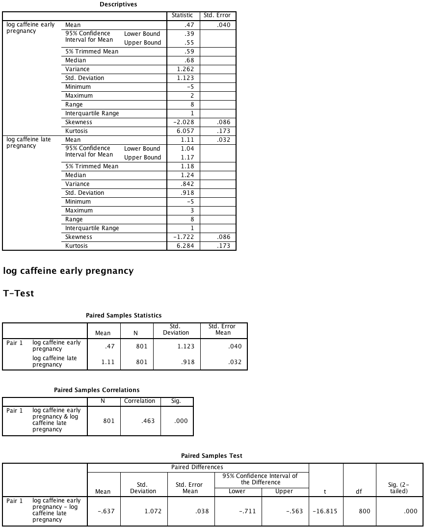
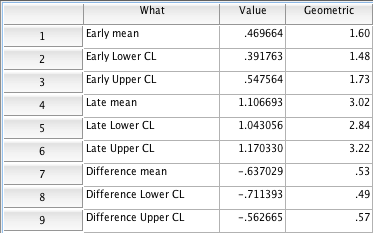
Figure 8.3 Instruction
Click here to show the instructions as text.SPSS does not have the ability to automatically calculate the geometric mean. The steps below show an way to get the tests on the geometric means and 95% confidence limits.
- Open the file.
- From the File menu choose Open > Data....
- Find the file cotinine.sav and open it.
- Tell SPSS to compute a natural log transformed version of serum creatinine.
- From the Transform menu choose Compute Variable....
- In the Target Variable: box type logCafEarly.
- In the Function group: box select Arithmetic.
- In the Functions and Special Variables: box double click Ln.
- Double click on cafearly.
- Click OK.
- Tell SPSS to compare the means of two related samples with a paired t-test.
- From the Analyze menu choose Compare Means > Paired-Samples T Test....
- Drag lcafearly to the Paired Variables: box.
- Drag lcaflate to the Paired Variables: box.
- Click OK.
- Tell SPSS to calculate means with 95% confidence limits.
- From the Analyze menu choose Descriptive Statistics > Explore....
- Drag lcafearly to the Dependent List: box.
- Drag lcaflate to the Dependent List: box.
- Click OK.
- Make a new dataset that will hold the transform of the mean and confidence limits.
- From the File menu choose New> Data.
- Click on Variable View (at the bottom of the window).
- Click the Name box/cell for the 1st row.
- Type What.
- Click the Type box/cell next to where you wrote What.
- Click on the ....
- Click on the String radio button.
- In the Characters: box type 25.
- Click OK.
- Click the Name box/cell for the 2nd row.
- Type Value .
- Click the Decimals box/cell for the 2nd row.
- Type 6.
- Click on Data View button (at the bottom of the window).
- In the first row, in the What cell, type Early mean.
- In the first row, in the Value cell, type 0.469664.
- In the second row, in the What cell, type Early Lower CL.
- In the second row, in the Value cell, type 0.391763.
- In the third row, in the What cell, type Early Upper CL.
- In the third row, in the Value cell, type 0.547564.
- In the fourth row, in the What cell, type Late mean.
- In the fourth row, in the Value cell, type 1.106693.
- In the fifth row, in the What cell, type Late Lower CL.
- In the fifth row, in the Value cell, type 1.043056.
- In the sixth row, in the What cell, type Late Upper CL.
- In the sixth row, in the Value cell, type 1.170330.
- In the seventh row, in the What cell, type Difference mean.
- In the seventh row, in the Value cell, type -0.637029.
- In the eighth row, in the What cell, type Difference Lower CL.
- In the eighth row, in the Value cell, type -0.711393.
- In the ninth row, in the What cell, type Difference Upper CL.
- In the ninth row, in the Value cell, type -0.562665.
- Tell SPSS to compute a do the antilog of the mean and confidence limits.
- From the Transform menu choose Compute Variable....
- In the Target Variable: box type Geometric.
- In the Function group: box select Arithmetic.
- In the Functions and Special Variables: box double click Exp.
- Double click on Value.
- Click OK.
The dataset already contains log versions of the caffeine variables. For your own data you do this:
By default, SPSS shows most statistcs with two decimal points. To see more, double click the results and then double click the values.
Figure 8.4 Output for a matched case-control analysis
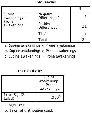
Figure 8.4 Instruction
Click here to show the instructions as text.
- Open the file.
- From the File menu choose Open > Data....
- Find the file sleep.sav and open it.
- Tell SPSS to do a sign test.
- From the Analyze menu choose Nonparametric Tests > Legacy Dialogs > 2 Related Samples....
- Drag proneawakenings to the Test Pairs: box.
- Drag supineawakenings to the Test Pairs: box.
- Click OK.
Box 8.7 Output for a Wilcoxon matched pairs test

Box 8.7 Instruction
Click here to show the instructions as text.
SPSS instructions go here
Figure 8.5 Output for a matched case-control analysis
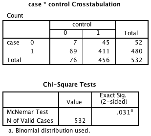
Figure 8.5 Instruction
Click here to show the instructions as text.
- Open the file.
- From the File menu choose Open> Data....
- Find the file casecontrol.sav and open it.
- Tell SPSS to do McNemar's Test.
- From the Analyze menu choose Descriptive Statistics > Crosstabs ....
- Drag case to the Rows(s) box.
- Drag control to the Column(s) box.
- Click Statistics....
- Check on the McNemar checkbox.
- Click Continue.
- Click OK.
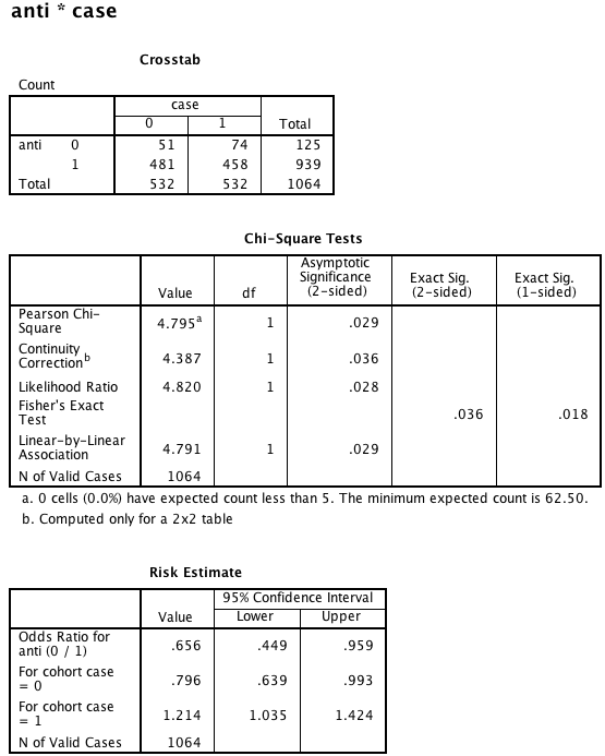
Box 8.10 Asthma case-control study
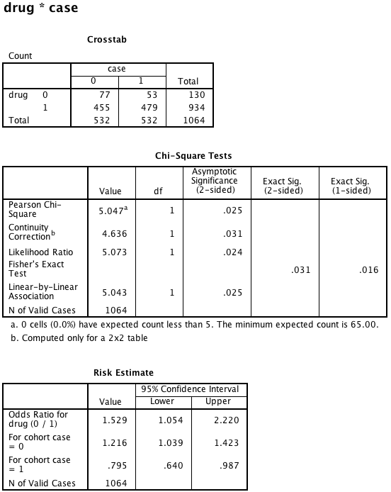
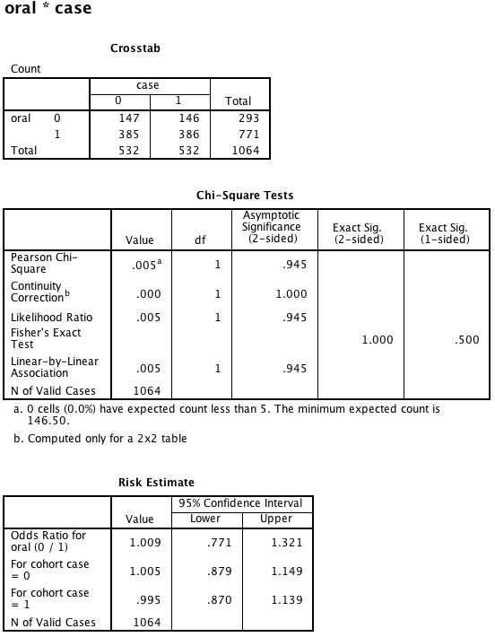
Box 8.10 Instruction
Click here to show the instructions as text.
- Open the file.
- From the File menu choose Open> Data....
- Find the file asthma.sav and open it.
- Tell SPSS to calculate Odds Ratios and Chi-square statistics.
- From the Analyze menu choose Descriptive Statistics > Crosstabs ....
- Drag drug, oral, and anti to the Rows(s) box.
- Drag case to the Column(s) box.
- Click Statistics....
- Check on the Chi-square checkbox.
- Check on the Risk checkbox.
- Click Continue.
- Click OK.
Figure 8.6 Output for McNemar’s test with ratio of paired proportions
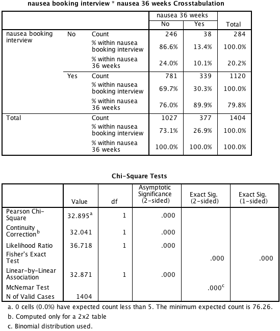
Figure 8.6 Instruction
Click here to show the instructions as text.
- Open the file.
- From the File menu choose Open > Data....
- Find the file cotinine.sav and open it.
- Tell SPSS to display words instead of code numbers for the nausea variables.
- Select the window showing the cotinine dataset.
- Click on Variable View (at the bottom of the window).
- Click the Values box/cell next to the nausea1 variable.
- Click on the ....
- Type 0 in the Values box.
- Type No in Label box .
- Click Add.
- Type 1 in the Values box.
- Type Yes in Label box .
- Click Add.
- Click OK.
- Click the Values box/cell next to the nausea2 variable.
- Click on the ....
- Type 0 in the Values box.
- Type No in Label box .
- Click Add.
- Type 1 in the Values box.
- Type Yes in Label box .
- Click Add.
- Click OK.
- Tell SPSS to do McNemar's Test.
- From the Analyze menu choose Descriptive Statistics > Crosstabs ....
- Drag nausea1 to the Rows(s) box.
- Drag nausea1 to the Column(s) box.
- Click Statistics....
- Check on the Chi-square checkbox.
- Check on the McNemar checkbox.
- Click Continue.
- Click Cells....
- In the Percentages section Check on the Row checkbox.
- In the Percentages section Check on the Column checkbox.
- Click Continue.
- Click OK.