Home > Output
Chapter 9: Analysing relationships between variables using STATA
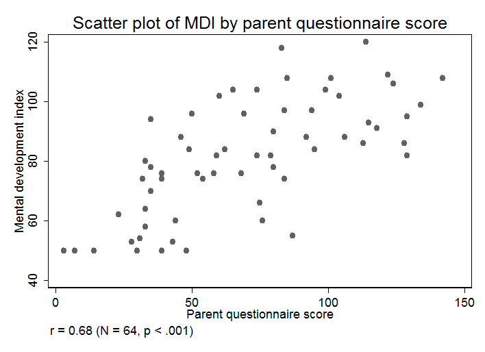
Figure 9.1 Scatterplot for two variables
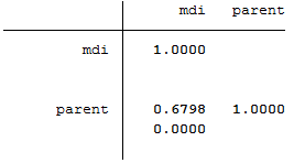
Figure 9.2 Output for Pearson’s correlation
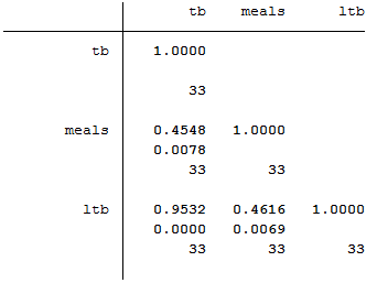
Box 9.3 Presenting the results for Pearson’s correlation


Figure 9.1, Figure 9.2 and Box 9.3 Code

Click here to show code as text
use "C:\Projects\Books\Presenting\data\stataData\screening.dta", clear

sum mdi parent

pwcorr mdi parent, sig

ci2 mdi parent, corr

twoway (scatter mdi parent, msymbol(circle_hollow)), ylabel(40(20)140) ///
xtitle(Parent questionnaire score) xscale(range(-1 2)) xlabel(0(50)150, valuelabel noticks) ///
title(Scatter plot of MDI by parent questionnaire score) caption(r = 0.68 (N = 64, p < .001))
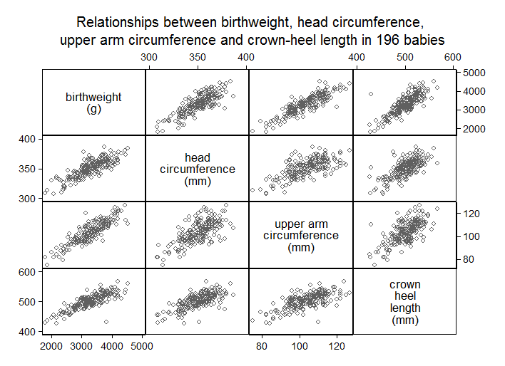
Figure 9.3 Scatterplots for several variables

Figure 9.3 Code

Click here to show code as text
use "C:\Projects\Books\Presenting\data\stataData\babyanth.dta", clear

gen ind=1 if  weight!=. &  head!=. &  arm!=. &  length!=.
label variable ind "indicator for complete cases"


graph matrix weight head arm length if ind==1, msymbol(circle_hollow) ///
	title("Relationships between birthweight, head circumference, ", size(medium)) ///
	subtitle("upper arm circumference and crown-heel length in 196 babies", size(medium))
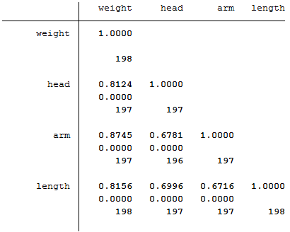
Figure 9.4 Calculating several correlations

Figure 9.4 Code

Click here to show code as text
use "C:\Projects\Books\Presenting\data\stataData\babyanth.dta", clear

pwcorr weight head arm length, sig obs
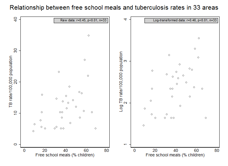
Figure 9.5 Presenting scatterplots (a) with skewed data and (b) where data are transformed


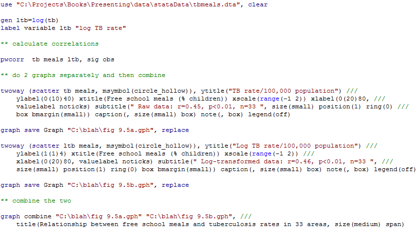
Figure 9.5 Code

Click here to show code as text
use "C:\Projects\Books\Presenting\data\stataData\tbmeals.dta", clear

gen ltb=log(tb)
label variable ltb "log TB rate"

** calculate correlations

pwcorr  tb meals ltb, sig obs

** do 2 graphs separately and then combine

twoway (scatter tb meals, msymbol(circle_hollow)), ytitle("TB rate/100,000 population") ///
	ylabel(0(10)40) xtitle(Free school meals (% children)) xscale(range(-1 2)) xlabel(0(20)80, ///
	valuelabel noticks) subtitle(" Raw data: r=0.45, p<0.01, n=33 ", size(small) position(1) ring(0) ///
	box bmargin(small)) caption(, size(small) box) note(, box) legend(off)

graph save Graph "C:\blah\fig 9.5a.gph", replace

twoway (scatter ltb meals, msymbol(circle_hollow)), ytitle("Log TB rate/100,000 population") ///
	ylabel(1(1)4) xtitle(Free school meals (% children)) xscale(range(-1 2)) ///
	xlabel(0(20)80, valuelabel noticks) subtitle(" Log-transformed data: r=0.46, p<0.01, n=33 ", ///
	size(small) position(1) ring(0) box bmargin(small)) caption(, size(small) box) note(, box) legend(off)

graph save Graph "C:\blah\fig 9.5b.gph", replace

** combine the two

graph combine "C:\blah\fig 9.5a.gph" "C:\blah\fig 9.5b.gph", ///
	title(Relationship between free school meals and tuberculosis rates in 33 areas, size(medium) span)
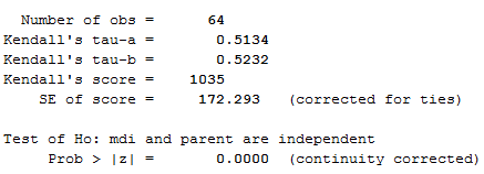
Figure 9.6 Output for a rank test

Figure 9.6 Code

Click here to show code as text
use "C:\Projects\Books\Presenting\data\stataData\screening.dta", clear

ktau mdi parent
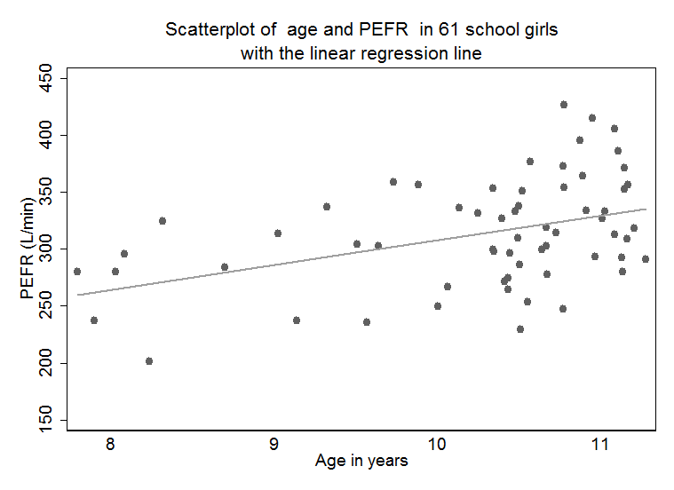
Figure 9.7 Scatterplot of two variables with linear regression line

Figure 9.7 Code

Click here to show code as text
use "C:\Projects\Books\Presenting\data\stataData\pefr.dta", clear

twoway (scatter pefr age) (lfit pefr age), ytitle(PEFR (L/min)) ylabel(150(50)450) xtitle(Age in years) ///
	xlabel(8(1)11, valuelabel noticks) title(Scatterplot of  age and PEFR  in 61 school girls, ///
	size(medium)) subtitle(with the linear regression line, size(medium) nobox) caption(, size(small) box) note(, box) legend(off)
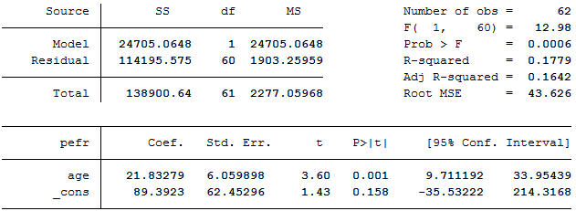
Figure 9.8 Output for simple regression


Figure 9.8

Click here to show code as text
use "C:\Projects\Books\Presenting\data\stataData\pefr.dta", clear

sum age pefr

regress pefr age
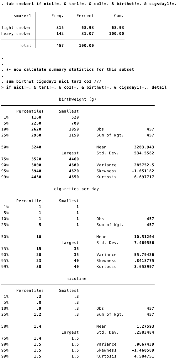
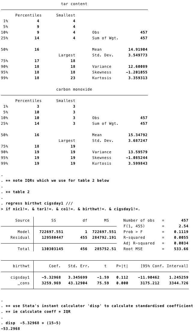
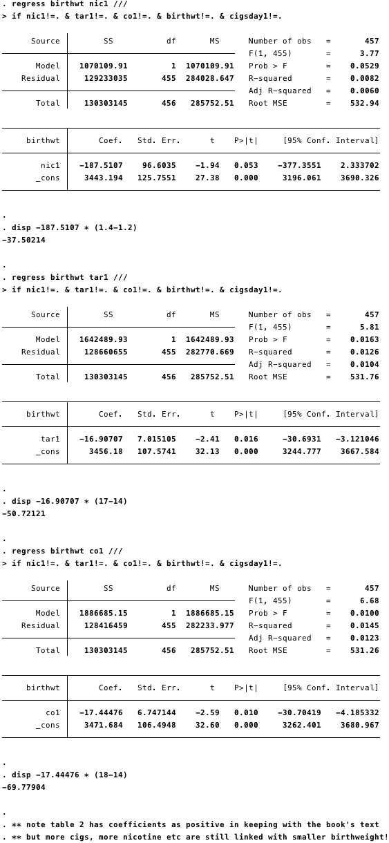
Box 9.11 Presenting the results for several predictor variables


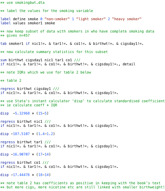
Box 9.11 Code

Click here to show code as text
use "C:\Projects\Books\Presenting\data\stataData\smokingbwt.dta", clear

** label the values for the smoking variable

label define smoke 0 "non-smoker" 1 "light smoker" 2 "heavy smoker"
label values smoker1 smoke

** now keep subset of data with smokers in who have complete smoking data
** gives n=457

tab smoker1 if nic1!=. & tar1!=. & co1!=. & birthwt!=. & cigsday1!=.

** now calculate summary statistics for this subset

sum birthwt cigsday1 nic1 tar1 co1 ///
if nic1!=. & tar1!=. & co1!=. & birthwt!=. & cigsday1!=., detail

** note IQRs which we use for table 2 below

** table 2

regress birthwt cigsday1 ///
if nic1!=. & tar1!=. & co1!=. & birthwt!=. & cigsday1!=.

** use Stata's instant calculator 'disp' to calculate standardised coefficient
** ie calculate coeff * IQR

disp  -5.32968 * (15-5)

regress birthwt nic1 ///
if nic1!=. & tar1!=. & co1!=. & birthwt!=. & cigsday1!=.

disp -187.5107 * (1.4-1.2)

regress birthwt tar1 ///
if nic1!=. & tar1!=. & co1!=. & birthwt!=. & cigsday1!=.

disp -16.90707 * (17-14)

regress birthwt co1 ///
if nic1!=. & tar1!=. & co1!=. & birthwt!=. & cigsday1!=.

disp -17.44476 * (18-14)

** note table 2 has coefficients as positive in keeping with the book's text
** but more cigs, more nicotine etc are still linked with smaller birthweight!
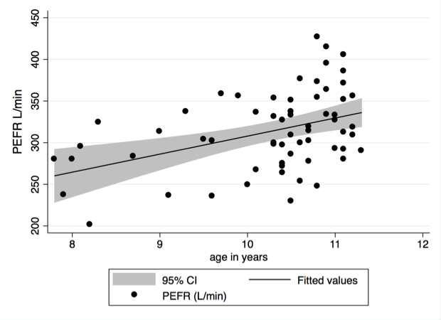
Box 9.14 Presentation of a regression line used for prediction
Figure 9.9 Scatterplot of two variables with linear regression line and 95% confidence intervals

Box 9.14 and Figure 9.9 Code

Click here to show code as text
use "C:\Projects\Books\Presenting\data\stataData\pefr.dta", clear

twoway (lfitci pefr age) (scatter pefr age), l1(PEFR L/min)

